Bayes nets (a type of Graphical Model) compactly represent how variables influence one another. Here's a Bayes net with five variables.

For simplicity, suppose these are all boolean (T/F) variables.
Notice that this diagram shows the causal structure of the situation, i.e. which events are likely to cause which other events. For example, we know that a virus can cause an upset stomach. Technically the design of a Bayes net isn't required to reflect causal structure. But they are more compact (therefore more useful) when they do.
For each node in the diagram, we write its probability in terms of the probabilities of its parents.

"Bad food" and "Virus" don't have parents, so we give them non-conditional probabilities. "Go to McKinley" and "Email instructors" have only one parent, so we need to spell out how likely they are for both possible values of the parent node.
"Upset stomach" has two parents, i.e. two possible causes. In this case, the two causes might interact. So we need to give a probability for every possible combination of the two parent values.
Two random variables A and B are independent iff P(A,B) = P(A) * P(B).
A and B are conditionally independent given C iff
P(A, B | C) = P(A|C) * P(B|C)
equivalently P(A | B,C) = P(A | C)
equivalently P(B | A,C) = P(B | C)
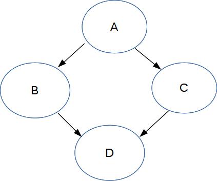
Here's a Bayes net modelling two effects with a common cause:
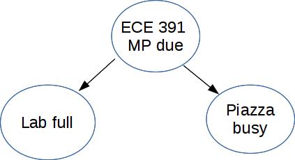
Busy piazza and a full lab aren't independent, but they are conditionally independent given that there's a project due.
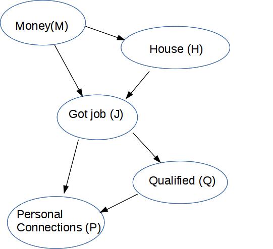
Here's an example of two causes jointly helping create a single effect:
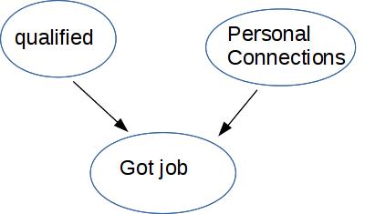
Being qualified is independent of having personal connections (more or less) But they aren't conditionally independent given that the person got the job. Supppose we know that they got the job but weren't qualified, then (given this model of the causal relationships) they must have personal connections. This is called "explaining away" or "selection bias."
A high-level point: conditional independence isn't some weakened variant of independence. Neither property implies the other.
Here's a causal chain, i.e. a sequence of events in which each causes the following one.
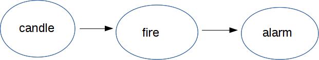
Candle and alarm are conditionally independent given fire. But they aren't independent, because P(alarm | candle) is much larger than P(alarm).
A set of independent variables generates a graphical model where the nodes aren't connected.

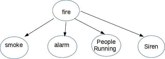
Naive Bayes can be modelled with a Bayes net that has one ancestor (cause) and a number of children (effects).
Recall from discrete math: a partial order orders certain pairs of objects but not others. It has to be consistent, i.e. no loops. So we can use it to draw a picture of the ordering with ancestors always higher on the page than descendents.
The arrows in a Bayes net are like a skeleton of a partial order: just relating parents to their children. The more general ancestor relationship is a true partial order.
For any set with a partial order, we can create a "topological sort." This is a total/linear order of all the objects which respects the partial order. That is, a node always follows its ancestors. Usually there is more than one possible topological sort and we don't care which one is chosen.
A Bayes net is a directed acyclic (no cycles) graph (called a DAG for short). So nodes are partially ordered by the ancestor/descendent relationships.
Each node is conditionally independent of its ancestors, given its parents. That is, the ancestors can ONLY influence node A by working via parents(A)
Suppose we linearize the nodes in a way that's consistent with the arrows (aka a topological sort). Then we have an ordered list of nodes \( X_1, ..., X_n\). Our conditional independence condition is then
For each k, \(P(X_k | X_1,...,X_{k-1}) = P(X_k | \text{parents}(X_k))\)
Suppose we have n variables. Suppose the maximum number of parents of any node in our Bayes net is m. Typically m will be much smaller than n.
We can build the probability for any specific set of values by working through the graph from top to bottom. Suppose (as above) that we have the nodes ordered \(X_1,...,X_n\). Then
\( P(X_1,...,X_n) = \prod_{k = 1}^n P(X_k | \text{parents}(X_k)) \)
\( P(X_1,...,X_n) \) is the joint distribution for all values of the variables.
In \( \prod_{k = 1}^n P(X_k | \text{parents}(X_k)) \), each term \( P(X_k | \text{parents}(X_k)) \) is the information stored with one node of the Bayes net.
Suppose we know the full full joint probability distribution for our variables and want to convert this to a Bayes net.. We can construct a Bayes net as follows:
Put the variables in any order \(X_1,\ldots,X_n\).
For k from 1 to nChoose parents(\(X_k\)) to contain all variables from \(X_1,\ldots,X_{k-1}\) that \(P(X_k)\) depends on.
This algorithm should work if applied to a joint distribution that was produced from a Bayes net. It is unlikely to work well if applied blindly to real-world data. There's two basic problems:
This sort of reconstruction would make the most sense in a context where you have a rough draft of the Bayes net and are using observed data to fine tune it.
Suppose we have a Bayes net that looks like this. This net contains 10 probability values: 1 each for Q and P, 2 each for M and H, 4 for J.

Suppose that we compute the corresponding joint distribution and then try to reconstruct the Bayes net using the above algorithms. If we use the variable order Q, P, J, M, H, then we'll get the above Bayes net back again.
But suppose we use the variable order M, H, J, Q, P. Then we proceed as follows:
M: no parents
H: isn't independent of M (they were only conditionally independent given J), so M is its parent
J: J isn't independent of M or H, nor is P(J | M,H) = P(J | H) so both of these nodes have to be its parents
Q: P(Q | J,M,H) = P(Q | J) so just list J as parent
P: probability depends on both J and Q
This requires that we store 13 probability numbers: 1 for M, 2 for H, 4 for J, 2 for Q, 4 for P.
So the choice of variable order affects whether we get a better or worse Bayes net representation. We could imagine a learning algorithm that tries to find the best Bayes net, e.g. try different variable orders and see which is most compact. In practice, we usually depend on domain experts to supply the causal structure.
As a result, Bayes nets make the most sense in certain domains. The AI designer should have strong sources of domain knowledge to guide the construction of the Bayes net. Each random variable should depend directly on only a small number of other (parent) variables. These assumptions would hold true, for example, in the domain of medical expert systems that help doctors make reliable diagnoses for unfamiliar diseases.
We'd like to use Bayes nets for computing most likely state of one node (the "query variable") from observed states of some other nodes. If we have information about the nodes at the top of the net, it's obvious how to compute probabilities for the state of nodes below them. However, we typically want to work from visible effects (e.g. money and house), through the intermediate ("unobserved") nodes, back to the causes (qualifications and personal connections).
For example:
In addition to the query and observed nodes, we also have all the other nodes in the Bayes net. These unobserved/hidden nodes need to be part of the probability calculation, even though we don't know or care about their values.
We'd like to do a MAP estimate. That is, figure out which value of the query variable has the highest probability given the observed effects. Recall that we use Bayes rule but omit P(effect) because it's constant across values of the query variable. So we're trying to optimize
\(\begin{eqnarray*} P(\text{ cause } \mid \text{ effect }) &\propto& P(\text{ effect } \mid \text{ cause }) P(\text{ cause }) \\ &=& P(\text{ effect },\text{ cause }) \end{eqnarray*} \)
So, to decide if someone was qualified given that we have noticed that they have money and a house, we need to estimate \( P(q \mid m,h) \propto P(q,m,h)\). We'll evaluate P(q,m,h) for both q=True and q=False, and pick the value (True or False) that maximizes P(q,m,h).
To compute this, \(P(q,m,h)\), we need to consider all possibilities for how J and P might be set. So what we need to compute is
\(P(q,m,h) = \sum_{J=j, P=p} P(q,m,h,p,j) \)
P(q,m,h,p,j) contains five specific values for the variables Q,M,H,P,J. Two of them (m,h) are what we have observed. One (q) is the variable we're trying to predict. We'll do this computation twice, once for Q=true and once for Q=false. The last two values (j and p) are bound by the summation.
Notice that \(P(Q=true,m,h)\) and \(P(Q=false,m,h)\) do not necessarily sum to 1. These values are only proportional to \(P(Q=true|m,h)\) and \(P(Q=false|m,h)\), not equal to them.
If we start from the top of our Bayes net and work downwards using the probability values stored in the net, we get
\(\begin{align}P(q,m,h) &= \sum_{J=j, P=p} P(q,m,h,p,j) \\ &= \sum_{J=j, P=p} P(q) * P(p) * P(j \mid p,q) * P(m \mid j) * P(h \mid j) \end{align} \)
Notice that we're expanding out all possible values for three variables (q,j,p). We look at both values for q because we're trying to decide between them. We're looking at all values of j and p because they are unobserved nodes. This will become a problem for problems involving more variables, because k binary variables have \(2^k \) possible value assignments.
Let's look at how we can organize our work. First, we can simplify the equation, e.g. move variables outside summations like this
\( P(q,m,h) = P(q) * \sum_{P=p} P(p) * \sum_{J=j} P(j \mid p,q) * P(m \mid j) * P(h \mid j) \)
Second, if you think through that computation, we'll have to compute \(P(j \mid p,q) * P(m \mid j) * P(h \mid j) \) four times, i.e. once for each of the possible combinations of p and j values.
But some of the constituent probabilities are used by more than one branch. E.g. \( P(h \mid J=true) \) is required by the branch where P=true and separately by the branch where P=false. Se we can save significant work by caching such intermediate values so they don't have to be recomputed. This is called memoization or dynamic programming.
If work is organized carefully (a long story), inference takes polynomial time for Bayes nets that are "polytrees." A polytree is a graph that has no cycles if you consider the edges to be non-directional (i.e. you can follow the arrows backwards or forwards).
But what if our Bayes net wasn't a polytree?
If your Bayes net is not a polytree, the junction tree algorithm will convert it to a polytree. This can allow efficient inference for a wider class of Bayes nets.
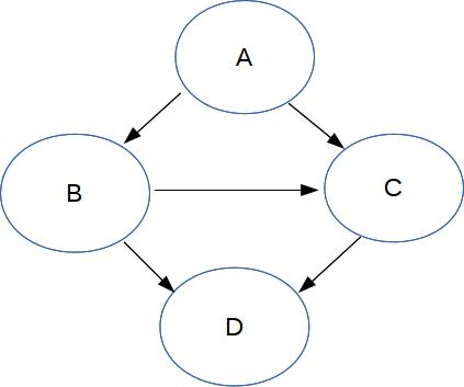
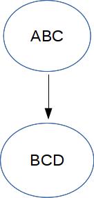
At a very high level, this algorithm first removes the directionality on the edges of the diagram. It then adds edges between nodes which aren't directly connected but are statistically connected (e.g. parents with a common child). This is called "moralization." It also adds additional edges to break up larger cycles (triangulaization). Fully-connected groups of nodes (cliques) are then merged into single nodes.
|
\(\rightarrow \) Moralize \(\rightarrow \) |
|
|
|
\(\rightarrow \) Merge cliques into single nodes \(\rightarrow \) |
|
