The high level classification model is simple, but a lot of details are required to get high quality results. We're now going to look at the details of why some challenges arrise and what tricks may be required to make Naive Bayes work well for text classification. Be aware that we're now talking about tweaks that might help for one application and hurt performance for another. "Your mileage may vary." For a typical example of the picky detail involved in this data processing, see the methods section from a word cloud generator project.
Our first job is to produce a clean string of words, suitable for use in the classifier. Suppose we're dealing with a language like English. Then we would need to
This process is called tokenization. Format features such as punctuation and capitalization may be helpful or harmful, depending on the task. E.g. it may be helpful to know that "Bird" is different from "bird," because the former might be a proper name. Similarly, "color" vs. "colour" might be a distraction or an important cue for distinguishing US from UK English. Does the difference between "student" and "students" matter? So "normalize" may either involve throwing away the information or converting it into a format that's easier to process.
Sometimes a word may have enough internal structure that it's best to divide it into multiple words. This happens somewhat in English, e.g. "moonlight". However, when English combines words without a hyphen or space, the compound word frequently has a special meaning different from its two pieces, e.g. "baseball".
Some other languages make much more use of compounding. E.g. German famously creates very long words where the overall meaning is the sum of the parts. For example "Wintermantel" is formed from into "winter" (winter) and "mantel" (coat). Our classifier may perform better if such words are divided by a "word segmenter".
In some applications, researchers have handled word endings by making them into separate words. The developers of the "Penn Treebank" found this useful in being able to form syntax trees, rather than just extract topic information. Here's two approaches to normalizing the word "student's":
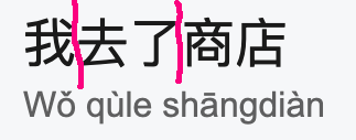
Some other languages do not put spaces between words. For example, "I went to the store" is written this way in Chinese

The sentence is written as a string of characters, each representing one syllable (below). But many pairs of characters (sometimes longer sequences) have meanings that are hard to predict from their pieces. Another meaning of the phrase "word segmenter" in computational language understanding is an algorithm that divides a string of letters or characters into conveniently sized meaningful chunks. The output might look like this:
As a general thing, the intended language processing application determines the appropriate size of the output tokens.
Classification algorithms frequently ignore very frequent and very rare words. Very frequent words ("stop words") often convey very little information about the topic. So they are typically deleted before doing a bag of words analysis.
Stop words in text documents are typically function words, such as "the", "a", "you", or "in". In transcribed speech, we also see
However, whether to ignore stop words depends on the task. Stop words can provide useful information about the speaker's mental state, relation to the listener, etc. See James Pennebaker "The secret life of pronouns". He and his colleagues have found, for example, that when there is a difference in status between the two people in a conversation, the subordinate is more likely to use the first-person singular ("I") pronoun. The higher-ranked person is more likely to use the first-person plural ("we") and second person ("you") pronouns.
Rare words include words for uncommon concepts (e.g. armadillo), proper names, foreign words, obsolete words (e.g. abaft), numbers (e.g. 61801), and simple mistakes (e.g. "Computer Silence"). Words that occur only one (hapax legomena) often represent a large fraction (e.g. 30%) of the word types in a dataset. Rare words cause two problems
Rare words may be deleted before analyzing a document. More often, all rare words are mapped into a single placeholder value (e.g. UNK). This allows us to treat them all as a single item, with a small but non-zero chance of being observed.
Smoothing assigns non-zero probabiities to unseen words. Since all probabilities have to add up to 1, this means we need to reduce the estimated probabilities of the words we have seen. Think of a probability distribution as being composed of stuff, so there is a certain amount of "probability mass" assigned to each word. Smoothing moves mass from the seen words to the unseen words.
Questions:
A good first approximation is that rare words should lose mass and unseen words should gain mass.
Some unseen words might be more likely than others, e.g. if it looks like a legit English word (e.g. boffin) it might be more likely than something using non-English characters (e.g. bête).
Smoothing is critical to the success of many algorithms, but current smoothing methods are witchcraft. We don't fully understand how to model the (large) set of words that haven't been seen yet, and how often different types might be expected to appear. Popular standard methods work well in practice but their theoretical underpinnings are suspect.
Performance of Laplace smoothing
A technique called deleted estimation (due to Jelinek and Mercer) can be used to directly measure these estimation errors and also do a more accurate version of smoothing.
Suppose that we divide a set of data into two halves. For each word (both halves together), we can compare the counts of the word in the two halves. Here's the start such a count table for the Wall Street Journal corpus.
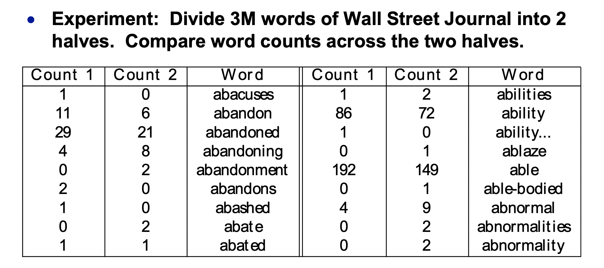
(from Mark Liberman
via Mitch Marcus)
Now, let's pick a specific count r in the first half. Suppose that \(W_1,...,W_n\) are the words that occur r times in the first half. We can estimate the corrected count for this group of words as the average of their counts in the second half. Specifically, suppose that \(C(W_k)\) is the count of \(W_k\) in the SECOND half of the dataset. Then
Corr(r) = \(\frac{\sum_{k=1}^n C(W_k)}{n}\)
Corr(r) predicts the future count for a word that has been seen r times in our training data. Deleted estimation has been shown to be more accurate than Laplace smoothing.
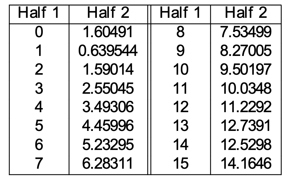
(from Mark Liberman
via Mitch Marcus)
Finally, let's make the estimate symmetrical. Let's assume for simplicity that both halves contain the same number of words (at least approximately). Then compute
Corr(r) as above
Corr'(r) reversing the roles of the two datasets
\( {\text{Corr}(r) +\text{Corr}'(r)} \over 2\) estimate of the true count for a word with observed count r
And now we can compute the probabilities of individual words based on these corrected counts. These corrected estimates still have biases, but not as bad as the raw counts were. The method assumes that our eventual test data will be very similar to our training data, which is not always true.
The Bag of Words model uses individual words as features, ignoring the order in which they appeared. Text classification is often improved by using pairs of words (bigrams) as features. Some applications (notably speech recognition) use trigrams (triples of words) or even longer n-grams. E.g. "Tony the Tiger" conveys much more topic information than either "Tony" or "tiger". In the Boulis and Ostendorf study of gender classification bigram features proved significantly significantly more powerful.
For n words, there are \(n^2\) possible bigrams. But our amount of training data stays the same. So the training data is even less adequate for bigrams than it was for single words.
Because training data is sparse, smoothing is a major component of any algorithm that uses n-grams. For single words, smoothing assigns the same probability to all unseen words. However, n-grams have internal structure which we can exploit to compute better estimates.
Example: how often do we see "cat" vs. "armadillo" on local subreddit? Yes, an armadillo has been seen in Urbana. But mentions of cats are much more common. So we would expect "the angry cat" to be much more common than "the angry armadillo". So
Idea 1: If we haven't seen an ngram, guess its probability from the probabilites of its prefix (e.g. "the angry") and the last word ("armadillo").
Certain contexts allow many words, e.g. "Give me the ...". Other contexts strongly determine what goes in them, e.g. "scrambled" is very often followed by "eggs".
Idea 2: Guess that an unseen word is more likely in contexts where we've seen many different words.
There's a number of specific ways to implement these ideas, largely beyond the scope of this course.