CS440/ECE448 Fall 2024, MP 9: Shallow Learning and Gradient Descent

Due: Monday, November 4, 11:59pm

I. Overview

In this assignment you will explore some fundamental concepts in Machine Learning. Namely you will fit functions to data to minimize some loss function. You will see a few different ways to compute such functions (analytically, gradient descent, and stochastic gradient descent). Using the same very simple implementation of gradient descent you will do linear regression, polynomial regression, inverse kinematics for a planar robot arm, and classification via logistic regression.

II. Getting Started

This assignment is structured more like a tutorial than an assignment. To get full credit you just need to pass all tests in tests.py and we highly recommend you work incrementally by following the notebook provided in mp9.ipynb. All instructions are in this notebook as well as in comments in mp9.py.

To get started on this assignment, download the template code. The template contains the following files and directories:

mp9.py: your main code goes here, this is the ONLY FILE you need to submit
tests.py: the tests in here (which are also called in the notebook) are identical to the ones in the autograder. You SHOULD NOT need to submit to gradescope to test your code.
mp9.ipynb: you should complete the assignment by working through the instructions in this python notebook. There is lots of code in this notebook to help you along.
data/: this folder contains some data for the last part of the assignment
planar_arm.py: some utilities for creating and drawing a planar robot arm for use in the inverse kinematics portion of the assignment
main.py: you can ignore this code if you work with the notebook, but this provides some utilities for running your code and generating nice plots (once your code works). There are some examples for how to run main.py in the notebook, and otherwise you can find all relevant parameters by typing python3 main.py --help

Notes:

You can open the provided python notebook in VSCode with the Jupyter extension or run it in browser by installing jupyter. If you’ve never worked with a python notebook before you may want to follow some quick online tutorial or come to office hours for help setting up.
Please DO NOT skip a function implementation as later parts may depend on it.
You have to write many functions but they are each very short.
One important goal for this assignment is to make you more familiar with doing linear algebra in python. This is a crucial skill for any kind of data science.

III. Assignment

1. Setting up linear regression

**Synthetic linear data with true line**

In this part of the assignment you will set up the necessary code for doing linear regression. Namely you will implement:

create_linear_data(num_samples, slope, intercept, x_range, noise)
get_simple_linear_features(x)
linear_prediction(x, A, get_modified_features)
mse_loss(y_pred, y_true)
compute_model_error(x, y, A, get_modified_features)

2. Analytical linear regression

**The more data we have with less noise the better our prediction is…**

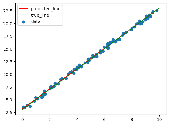
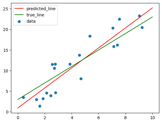
Now you will implement analytical linear regression which will compute parameters that minimize the mean squared error loss function

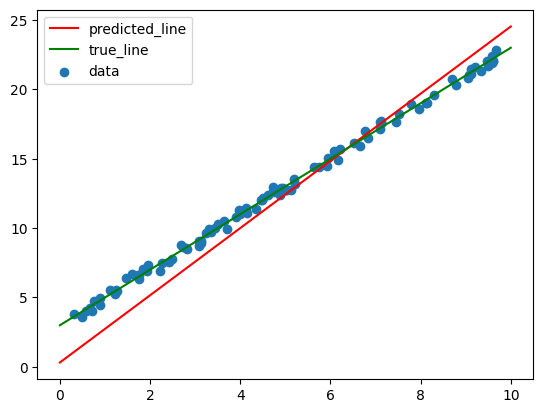
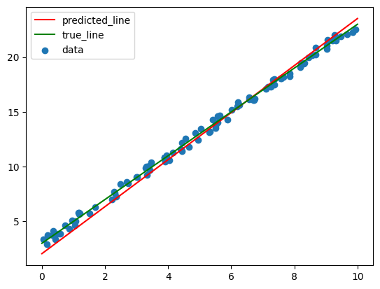
3. Gradient descent and stochastic gradient descent

On the left we have 10 iterations of gradient descent and on the right we have 10 epochs of stochastic gradient descent with a batch size of 10. Both had a learning rate of 0.01. Even though both methods did 10 passes through the data, SGD does better because every full pass through the data does more updates to the parameters (even though those updates were individually less precise).

Now you will implement a very simple version of the gradient descent algorithm given a function which computes the gradient with respect to the parameters.

Next you will implement a variation of the previous algorithm which uses a random ordering of subsets of the data to iteratively update parameters, instead of using the entire dataset at once for estimating the gradient.

4. Fitting sine data

**A linear function cannot fit this sinosoidal data…**

**If we transform our features to polynomial we can now fit the data!**

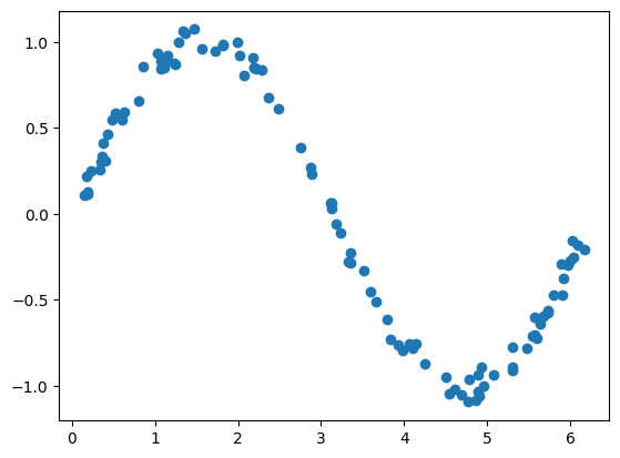
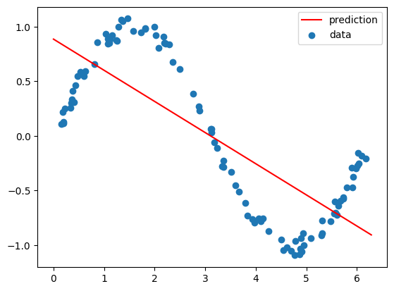
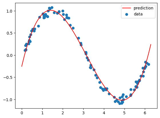
Now you will see how by transforming the input features into a new feature space (polynomial function of the input) you can use your previous linear regression code to fit a function to sine data.

5. Inverse kinematics

**We can use gradient descent to move an arm so that its tip is in a desired position. By modifying our loss function we can even make it avoid obstacles (i.e., do motion planning).**

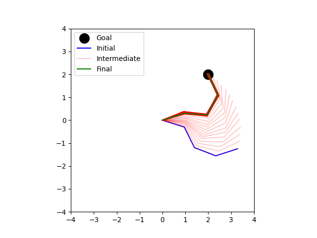
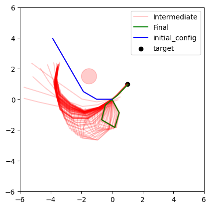
Now you will use gradient descent to iteratively update the configuration of a planar arm (meaning the joint angles) until the tip of the arm is in a desired position. You will estimate the direction for the update empirically, by sampling nearby configurations and choosing the local gradient direction.

6. Logistic regression

**We can find a linear separator by doing logistic regression using our get_simple_linear_features. With polynomial features we can correctly classify the data on the right.**

You will need to come up with your own features to correctly classify the third dataset above… On the left is what happens when we try degree 6 polynomial features. Can you come up with something that looks more like what we have on the right?

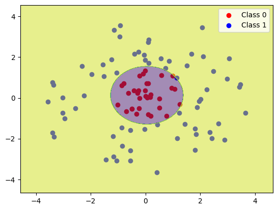
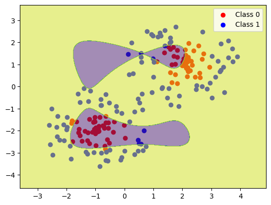
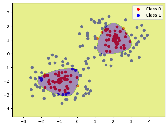
Finally, you will now do classification using gradient descent. This means implementing a new gradient for a new kind of model - logistic instead of linear. You will fit this model to data we provide (instead of you creating the data). Your current feature transforms (linear and polynomial) will be insufficient for fitting the third dataset we provide and so you will have to come up with your own feature transform.