 (from
Wikipedia)
(from
Wikipedia)
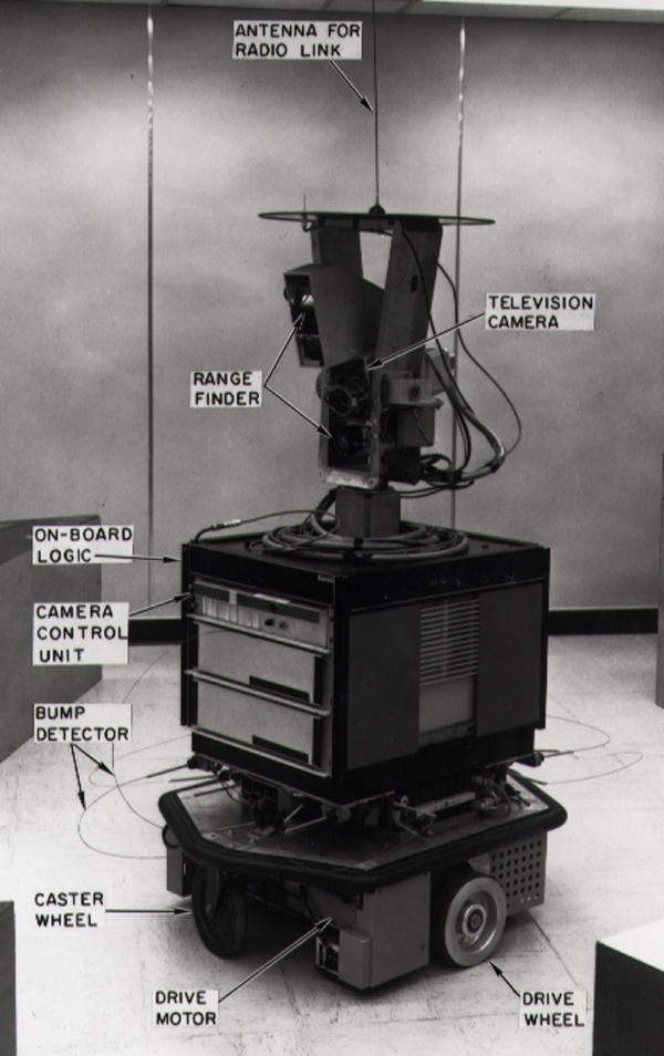
Even though Shakey was built 50 years ago, it still had the basic components of a mobile robot. That is:
Newer robots may also have features like
A skin-penetration sensor was used by a well-known sheep shearing robot (James Trevelyan, 1987) to make sure that any errors were corrected quickly.
Batteries are a surprisingly critical part of the design. Even now, they are heavy compared to how much power they deliver. So they can be a significant percentage of the robot's weight.
A robot usually has several redundant sensors because they fail in different ways, e.g. whiskers operate only at very short distances, IR sensors fail on dark surfaces.
There is a tradeoff between extra features and better safety. Robots working close to humans have to be less ambitious so that they are more reliably safe.
The big question for a mobile robot is how it moves:
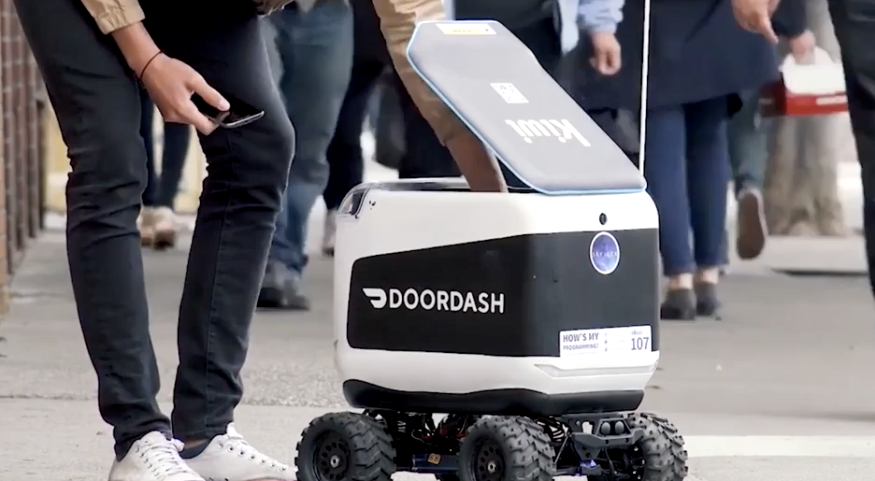
Food delivery robot from Techcrunch May 26, 2018 |

Waymo (Google) self-driving car |
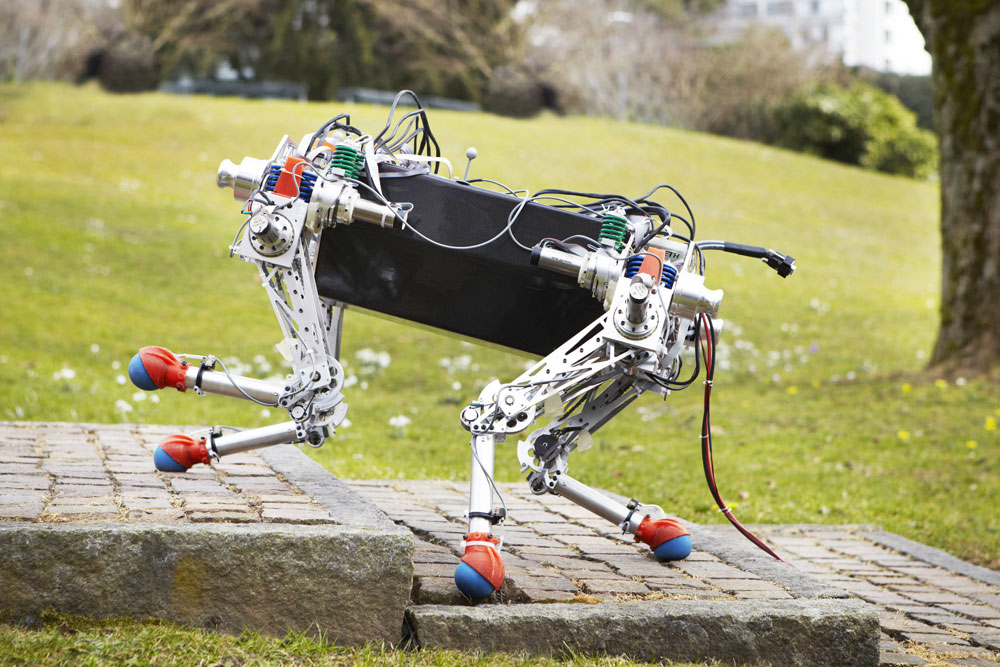
legged robot from ETH Zurich |
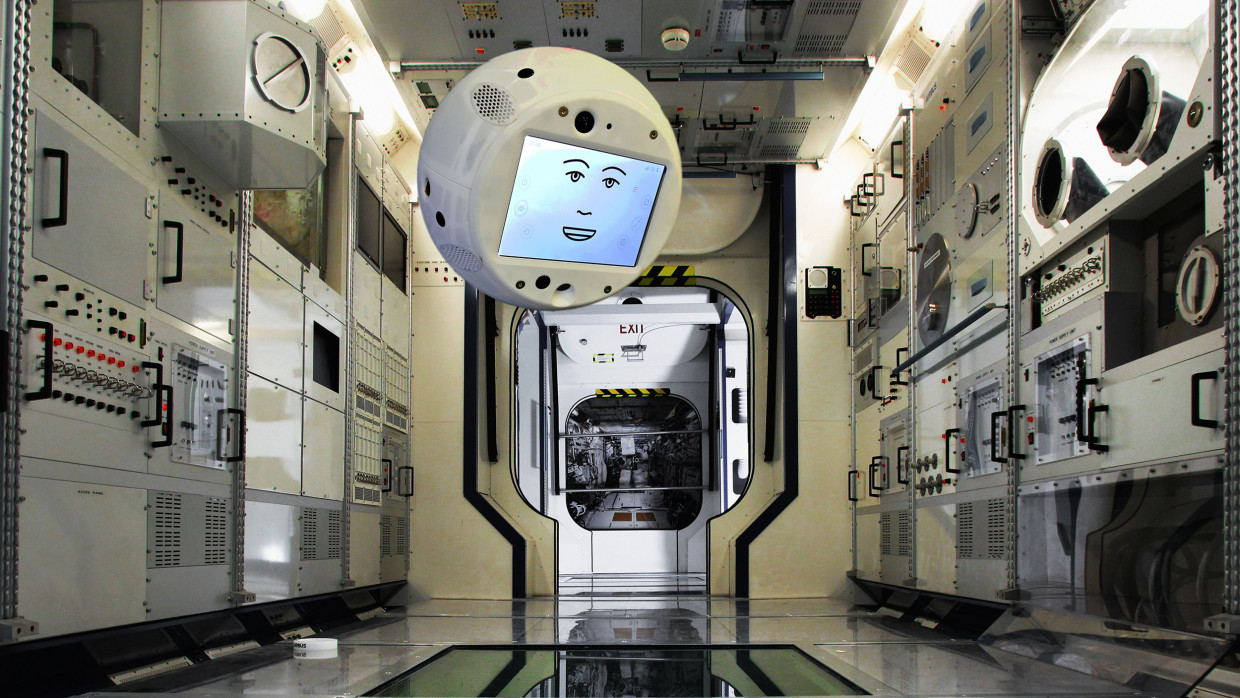
Cimon floating on the ISS from NBC |
Guard robot from The Telegraph |
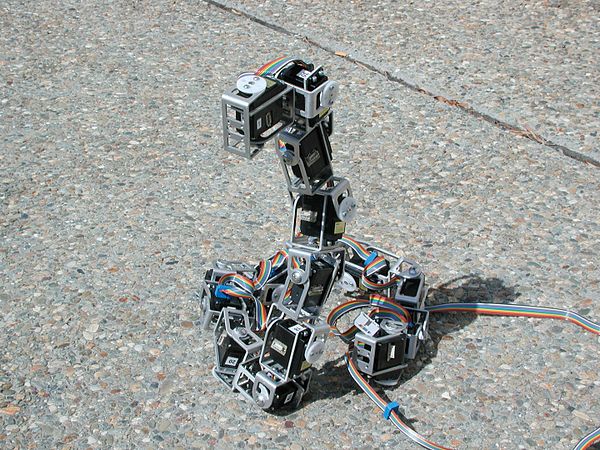
Snakebot from NASA |
|---|
Robots generate the best videos in the field.
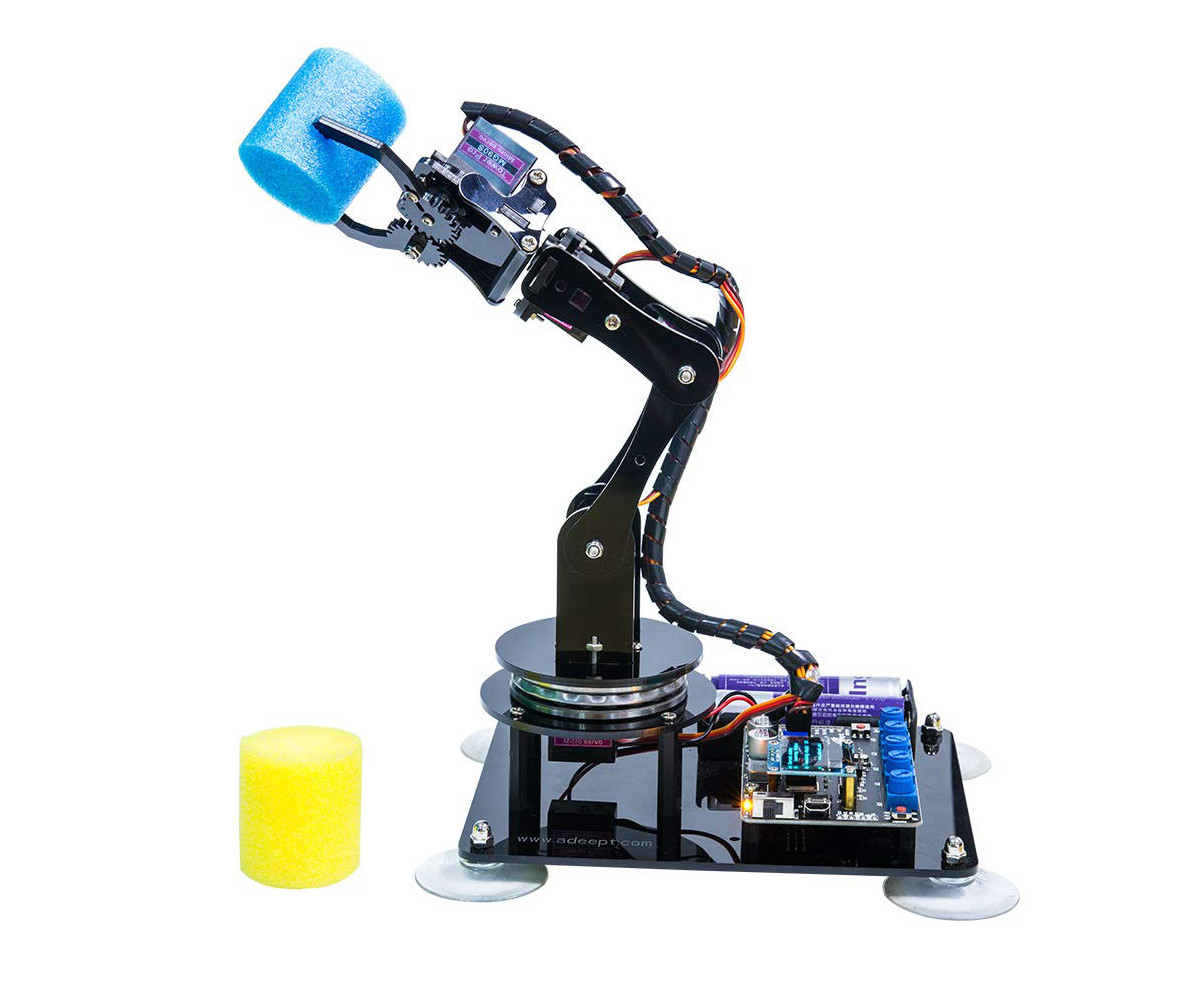 Adeept robot arm for Arduino (from Amazon)
Robots can also be jointed arms, mounted on a fixed base or a mobile one. This were originally used primarily for industrial assembly, due to safety concerns. As they have become smaller and more reliable, we also see human-facing applications.
Highlights of the Hannover MESSE 2017
Parts assembly: Allied-Technology.com Tabletop Demo of Small Parts Assembly
Some robots hang from the ceiling, e.g. this chef robot from Samsung:
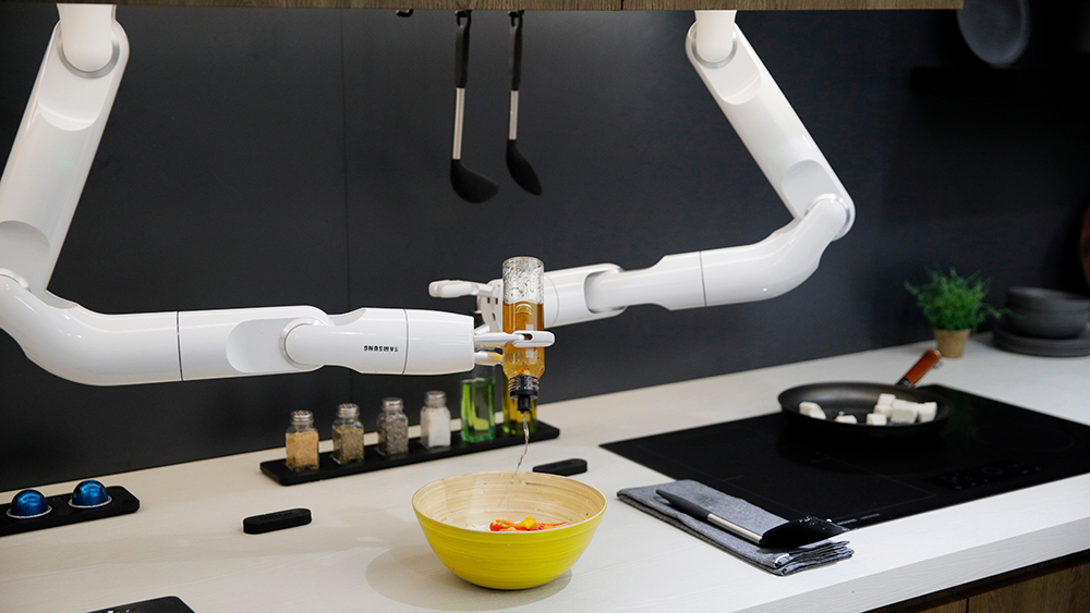 from
the Robb Report
from
the Robb Report
Samsung chef robot video at CES 2020
Planning motions of for jointed arms is made complex by the need to translate between real-world coordinates and joint angles. We'll see the details soon.
Also, very accurate positioning requires that links remain stiff, which ends up requiring very heavy robots for absurdly small payloads. E.g. a very accurate person-sized robot may have only a 10lb payload. Both high-level and low-level planning are more complicated when links may flex and/or there is significant error in positioning.
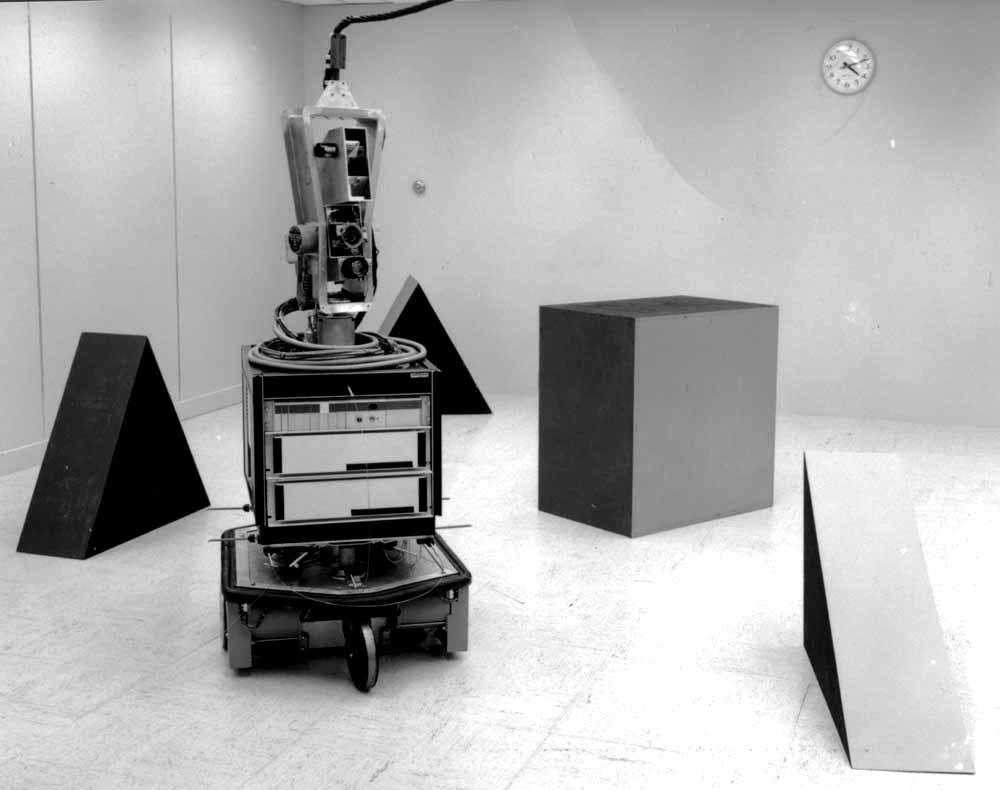
Very early robots such as Shakey moved around a world that was largely static and easy to figure out from camera images. Objects moved only when the robot made them move. (Any grad student helpers would be sneaking around behind its back.)
 (from
New Atlas)
(from
New Atlas)
As AI systems have gotten more capable, they have moved into more relaistic environments:
More complex planning problems happen when multiple robots need to work as a team, as in this video of U. Penn drones playing James Bond
Planning motions for robots isn't too difficult if the robot is very tiny, so we can approximate it as a point. However, that's usually not the case. So a key problem in robotics is
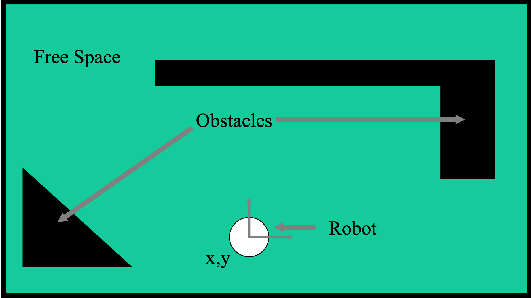
Where can the robot move when the robot has significant size?We'll model robot and obstacles as simple geometrical shapes to develop the ideas.
Suppose that we're moving a circular robot in 2D. We can simplify planning using the following idea:
Idea: expand obstacles so we can shrink robot to a point.
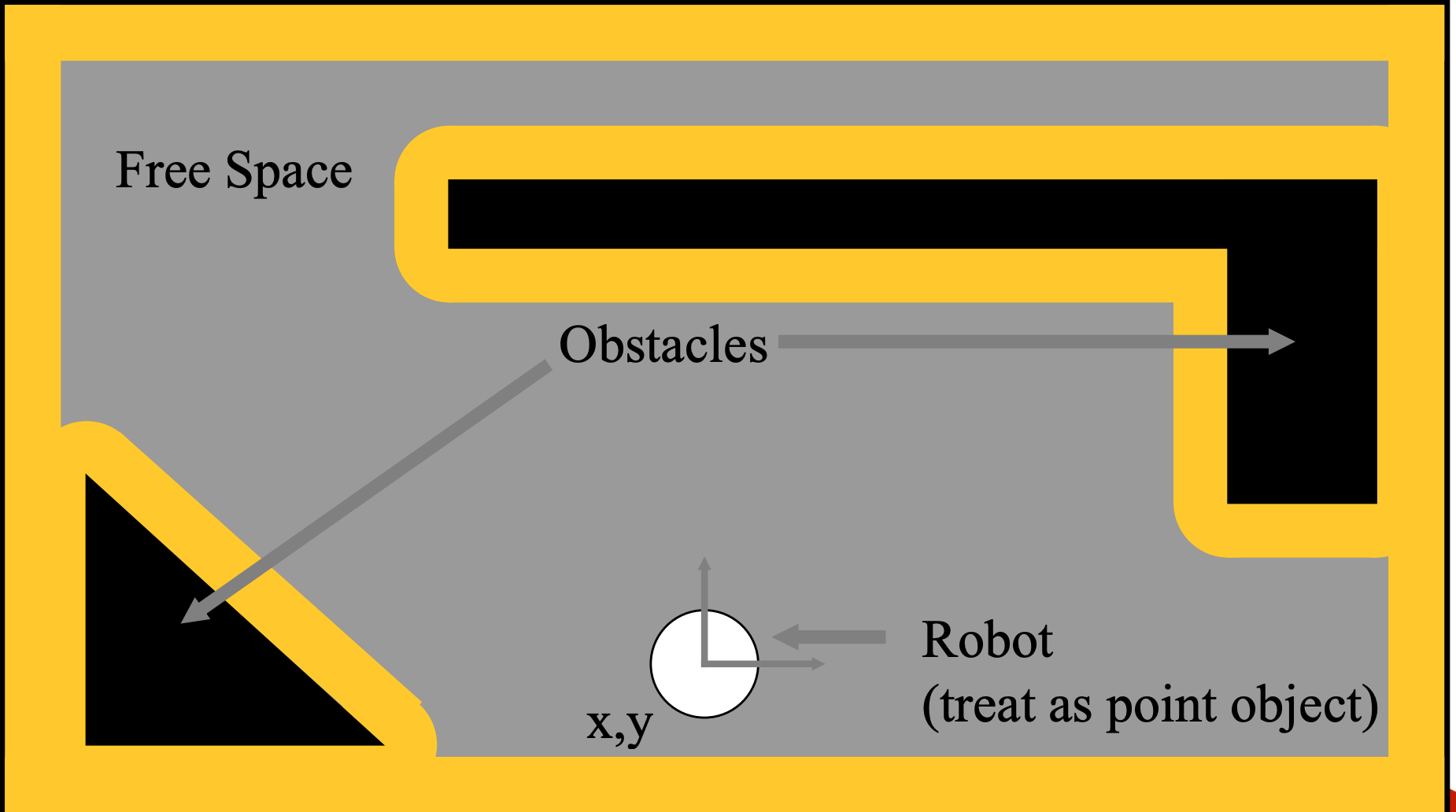
(from Howie Choset slides)
This modified space is called a configuration space. It shows all the possible positions for the center of the robot.
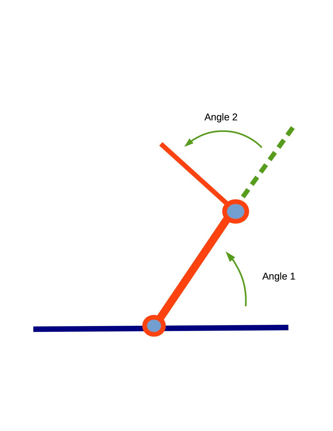
Another standard simple example is a robot arm with two links connected by rotating joints, like this:
To get a sense of how the arm can move around obstacles, play around with this 2-link robot simulator by Jeffrey Ichnowski. Or look at these pictures of a physical robot model .
Our high-level planning task is expressed in normal 2D coordinates, e.g. move the tip from one (x,y) location to another. However, we control the robot via the angles of the joints. These \((\alpha,\beta)\) pairs form a different 2D space, called the configuration space of the problem:
Big idea: do planning in configuration space (Lozano-Perez around 1980).
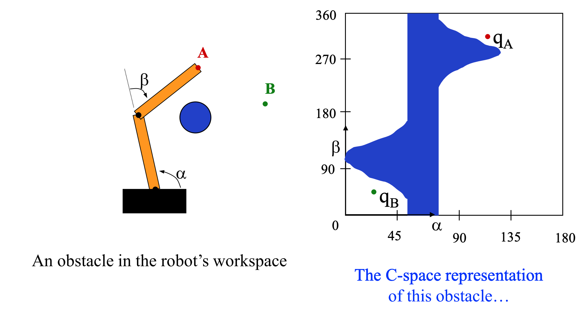
Here's an obstacle in a 2-link arm's configuration space (from Howie Choset). The x-axis of the configuration space diagram shows the angular position of the first/lower link in the arm. The y-axis shows the angular position of the second link The end of the arm is currently at A, corresponding to \(q_A\) in configuration space. We'd like to move the end of the arm to B. Howver, the obstacle in configuration space blocks all paths from \(q_A\) to \(q_B\). (Notice that the first joint can't rotate all the way around, since its values stop at 180. So this diagram doesn't wrap around.)
Here's the path of a 2-link arm in real space and configuration space (Howie Choset credited to Ken Goldberg): The starting and ending positions of the arm are shown in thicker red lines on the lefthand (real space) figure.
Notice that a goal in real space might correspond to more than one point in configuration space. For 2-link arm, many 2D points can be reached with the elbow pointing in two ways. For arms with more links, we can find multiple solutions to goals that specify the angle, as well as the position, of the hand. The pictures below show how a human can provide more than one way to put the hand at a particular position and orientation in 3D. The problem of going from a hand position back to (some) set of joint angles is called inverse kinematics.
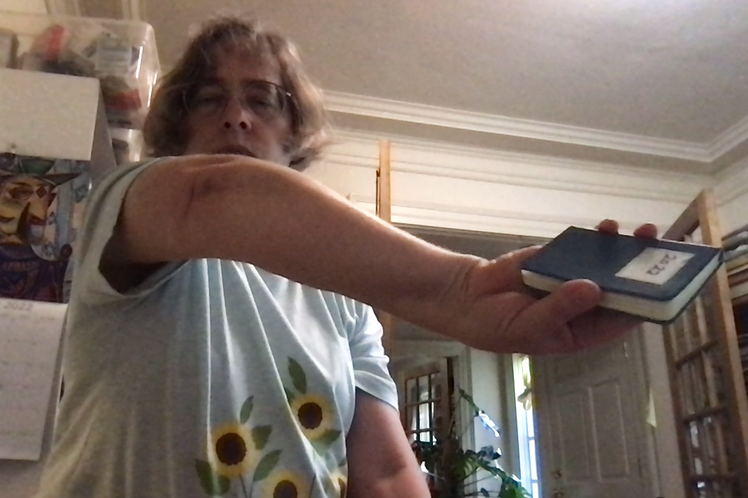
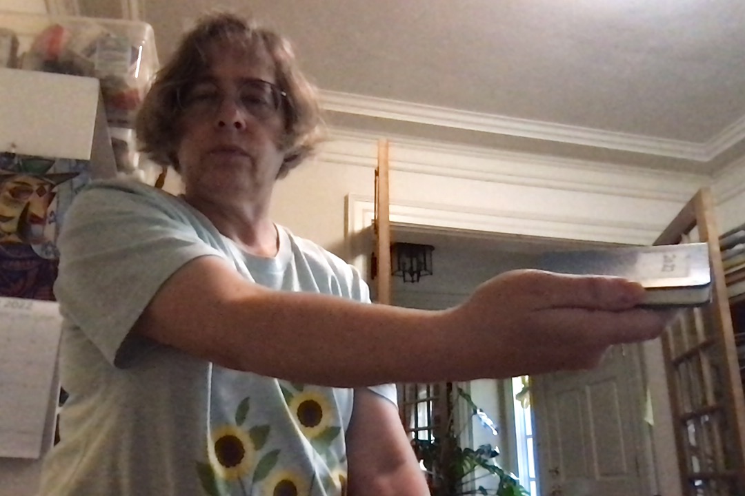
When there are multiple ways to get the business end of a robot arm into the right position and orientation, some may be more preferable. For example, some options may put a joint at the edges of its motion limits. Some may coordinate better with what the robot should be doing before and/or or after it's at that position.
The same mathematical system can be used to model a reverse system where the working end must be kept stable despite motion of what's supporting it. For example, this Kingfisher can keep its head in a fixed position while its feet hold onto a moving branch.
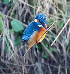
Kingfisher video from the Audobon Society
The figures above credited to Howie Choset came from Howie Choset, CMU 16-311, Spring 2018 and 16-735, Fall 2010. For more details, check out his book Principles of Robot Motion.
Fun book on collision detection by Jeff Thompson
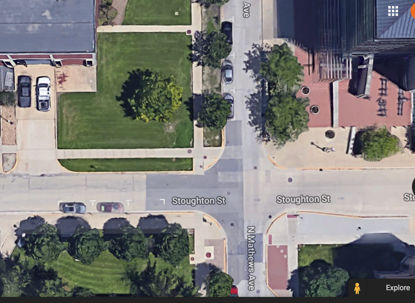 (from Google maps)
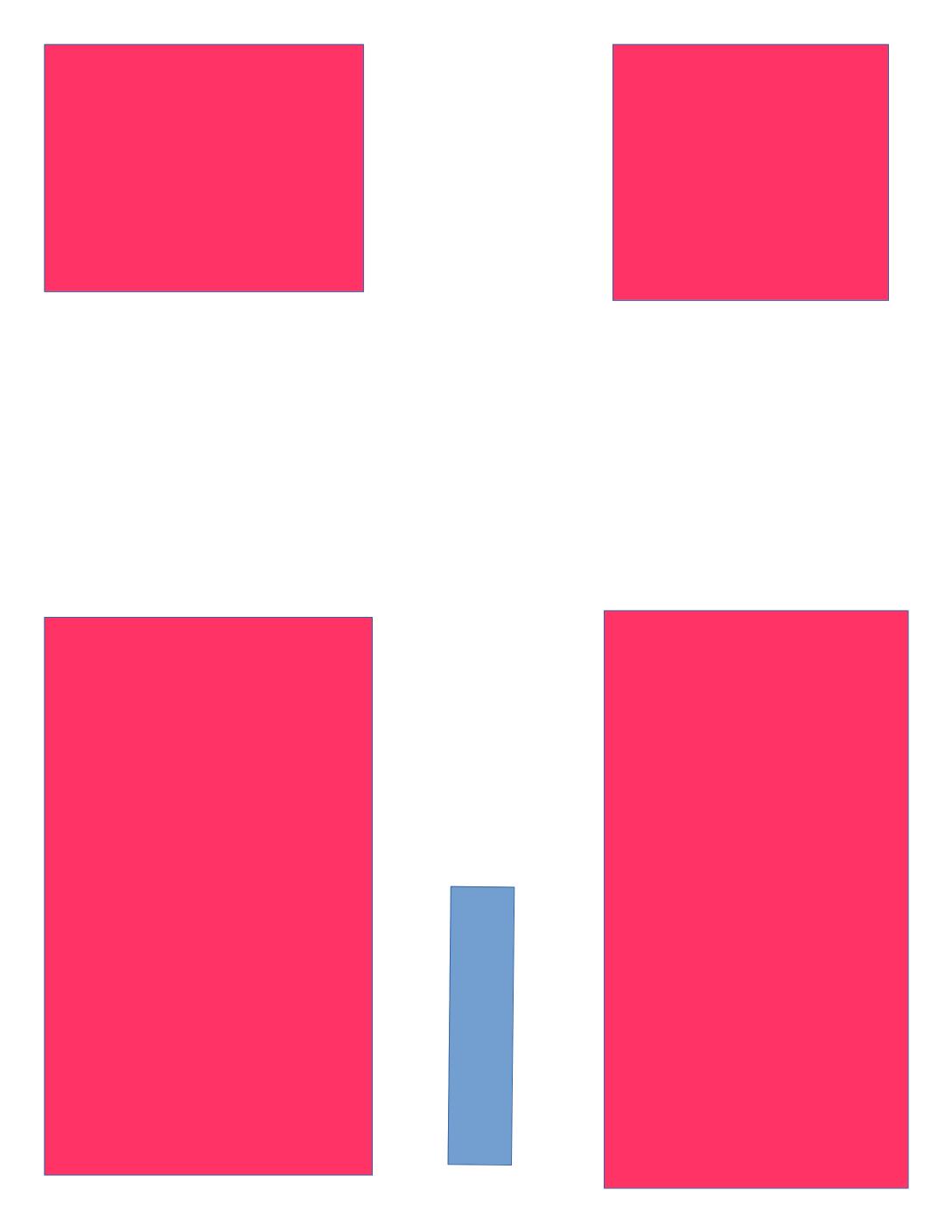
Now consider a polygonal robot moving around in 2D. For example, a car or truck might be moving around the roads near the Siebel Center shown in the areal view above. In the simplified map below , we have two crossing roads defined by four obstacles (red). The car (blue) can move forwards and rotate.
|
|
|
|
|
|
|---|
To specify the robot's position, we need to give its (x,y) position and also its orientation. So the robot's configuration space is three dimensional.
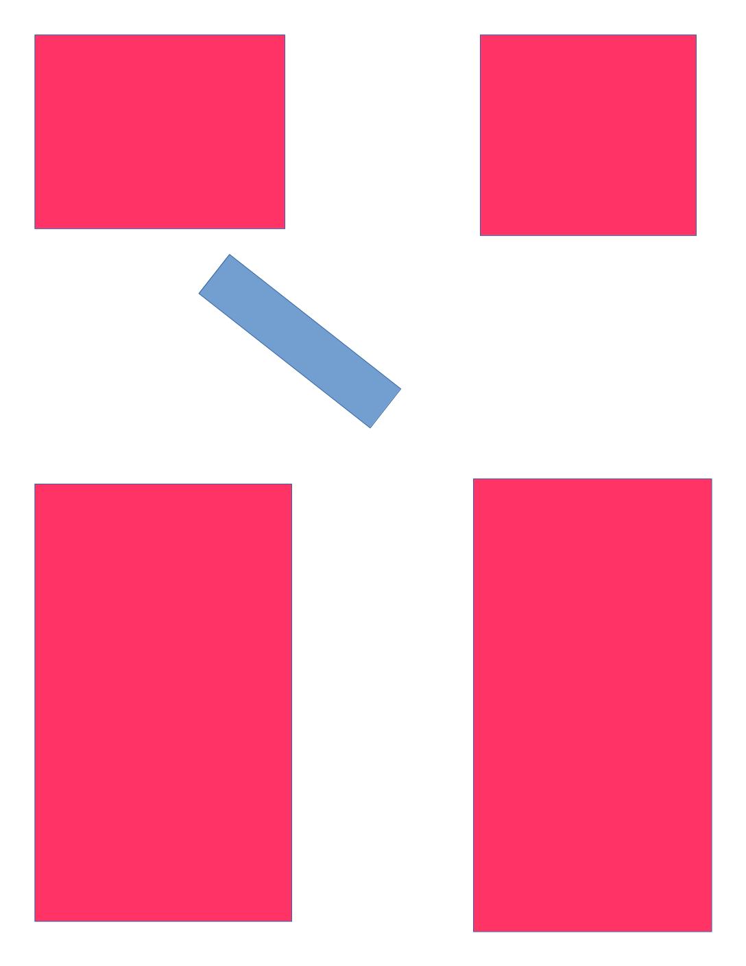
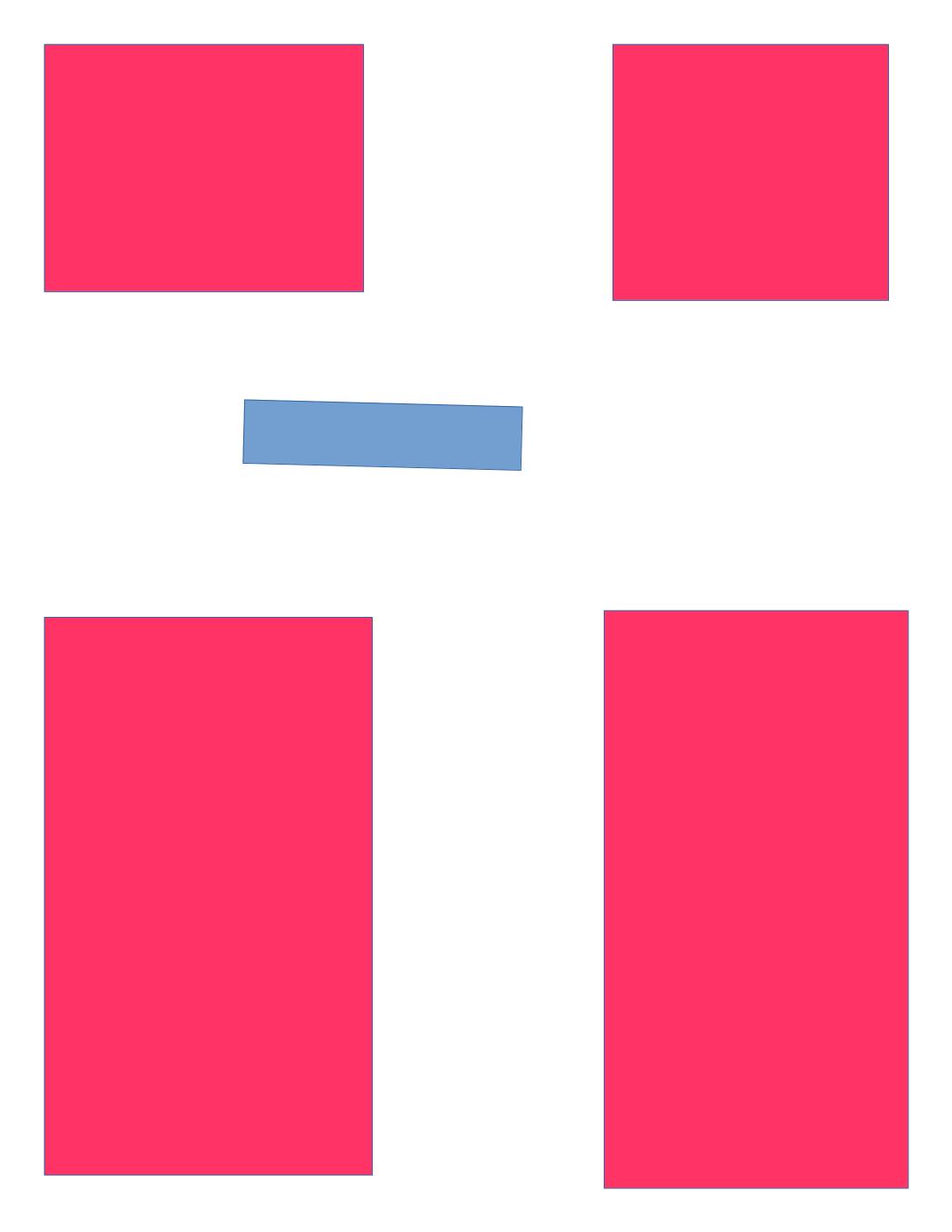
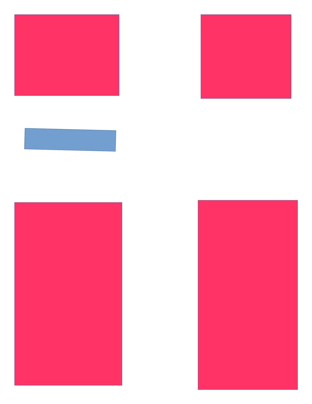
Here is the configuration space for a horizontal bar (red) moving around two vertical bars (gray) from Howie Choset.
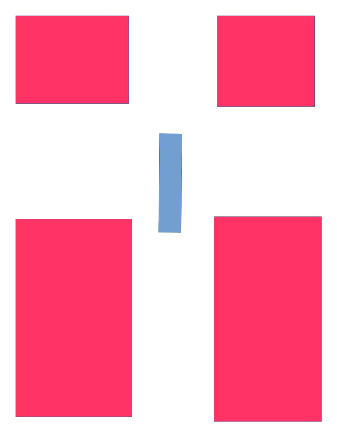
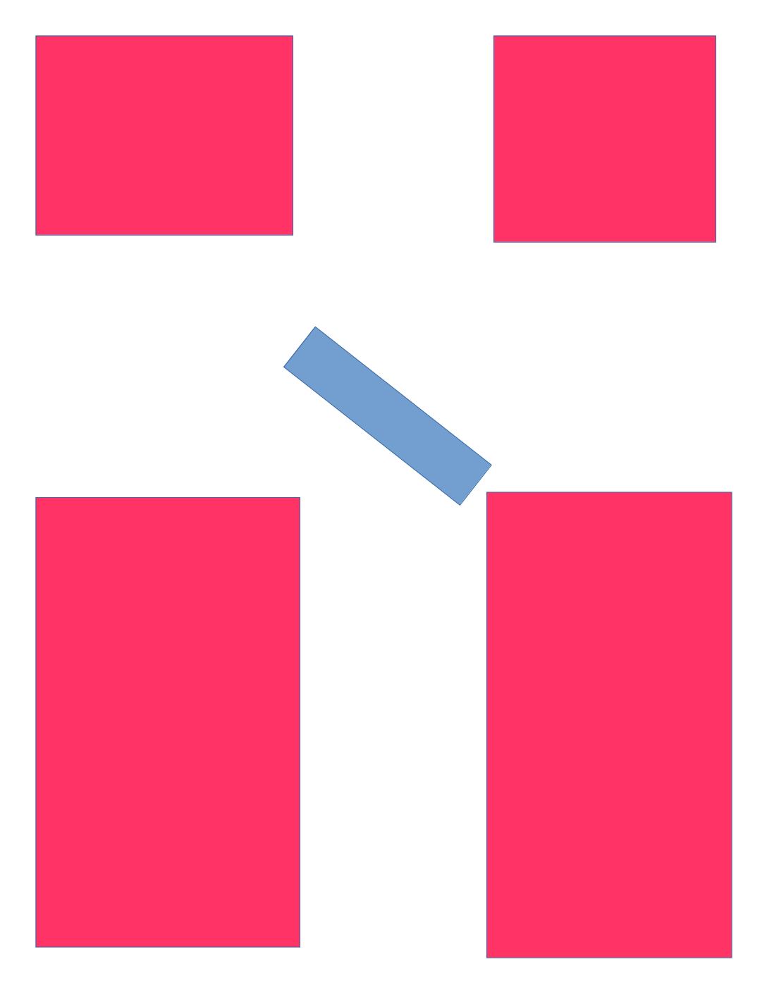
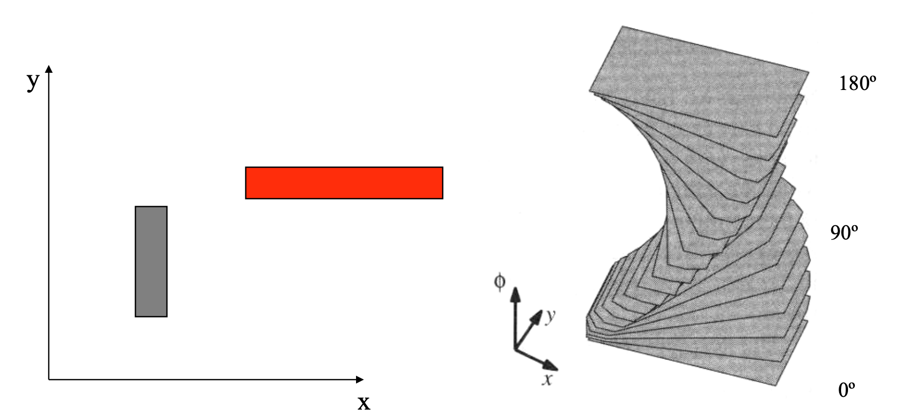
Now for the same bar in a diagonal orientation:
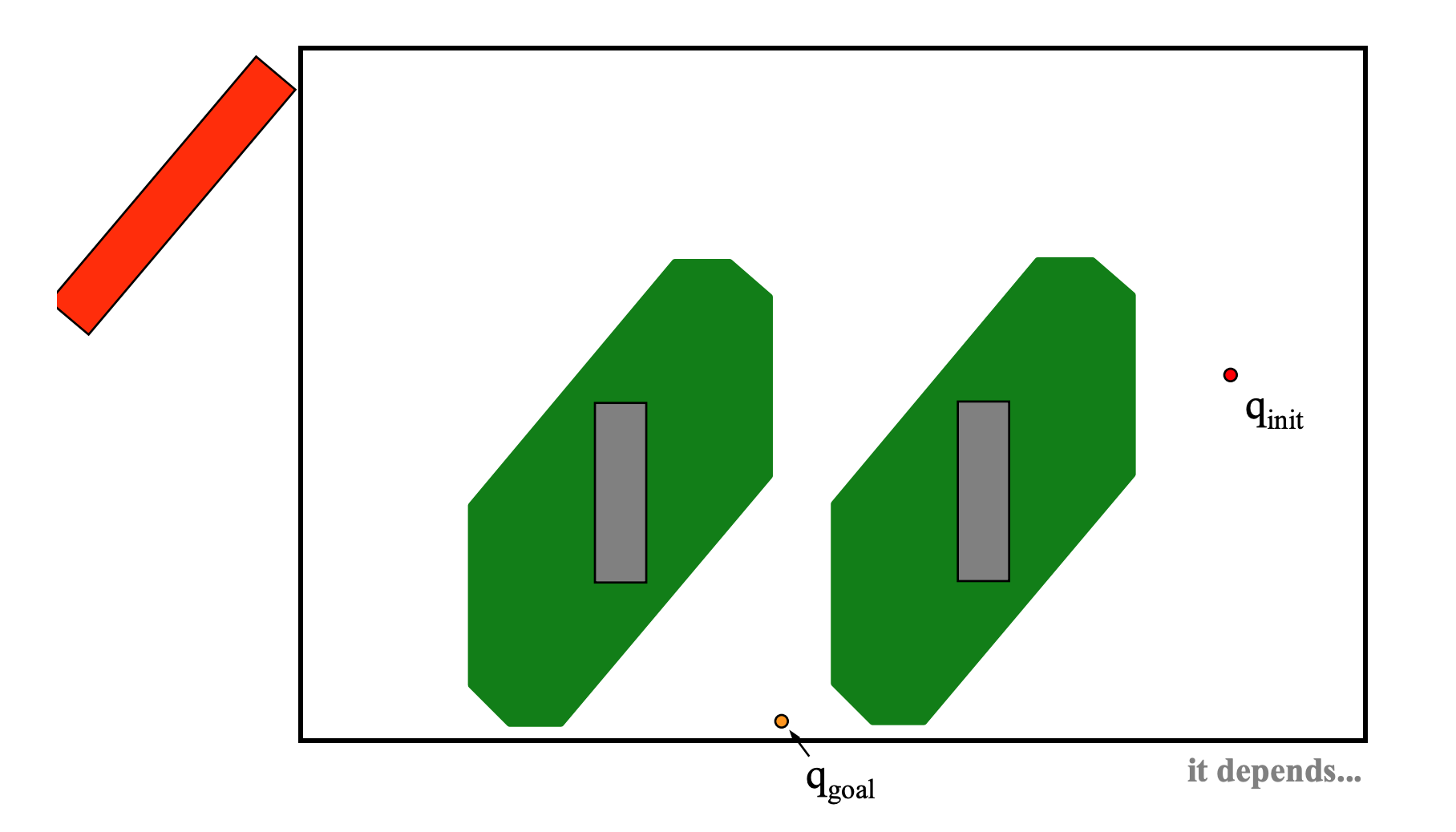
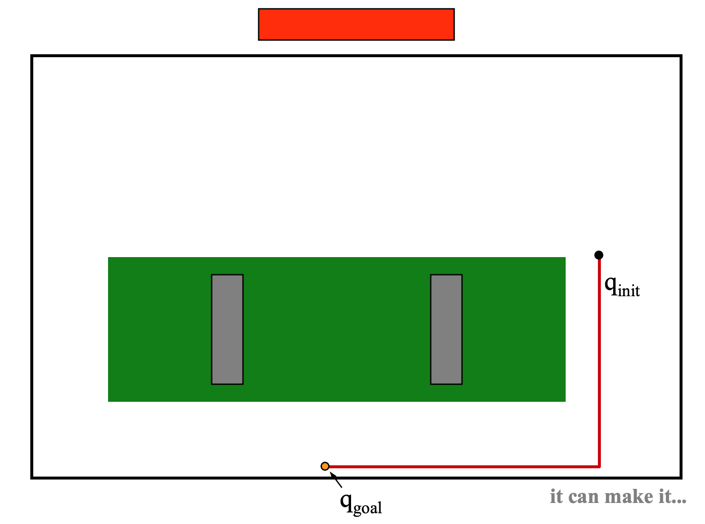
Finally, here is how a single vertical bar (gray) looks in the configuration of a red bar that can rotate as well as translate.
Here's an L-shaped object rotating to get through some tight doorways in 2D (from Howie Choset's slides). This kind of planning is quite difficult and can be computationally expensive.
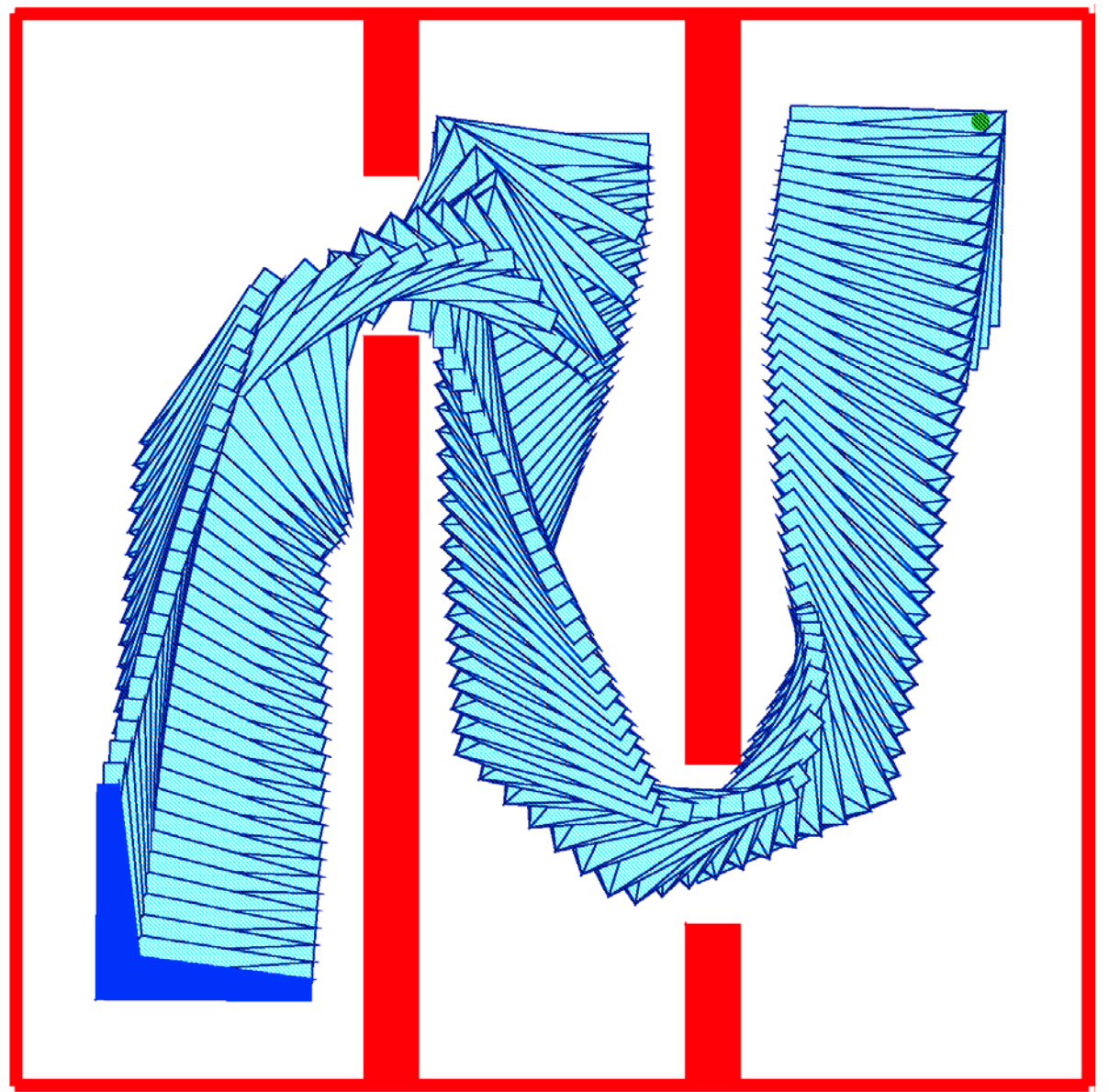
So this 2D problem with simple polygonal obstacles has a 3D configuration space with quite complex obstacles.
The dimensionality of the configuration space gets even larger in many real-world situations. For example, if we
How do we compute a path in a configuration space?
For simple 2D examples, e.g. MP 2, we can digitize the configuration space positions and use a digitized maze search algorithm. However, this approach scales very badly.
Normally we convert configuration space into a graph representation containing
These graph representations are compact and can be searched efficiently.
One graph-based approach uses vertices of objects as waypoints. Edges are straight lines connecting vertices. This "visibility graph" can be constructed incrementally, directly from a polygonal representation of the obstacles:
(Pictures from Choset again.)
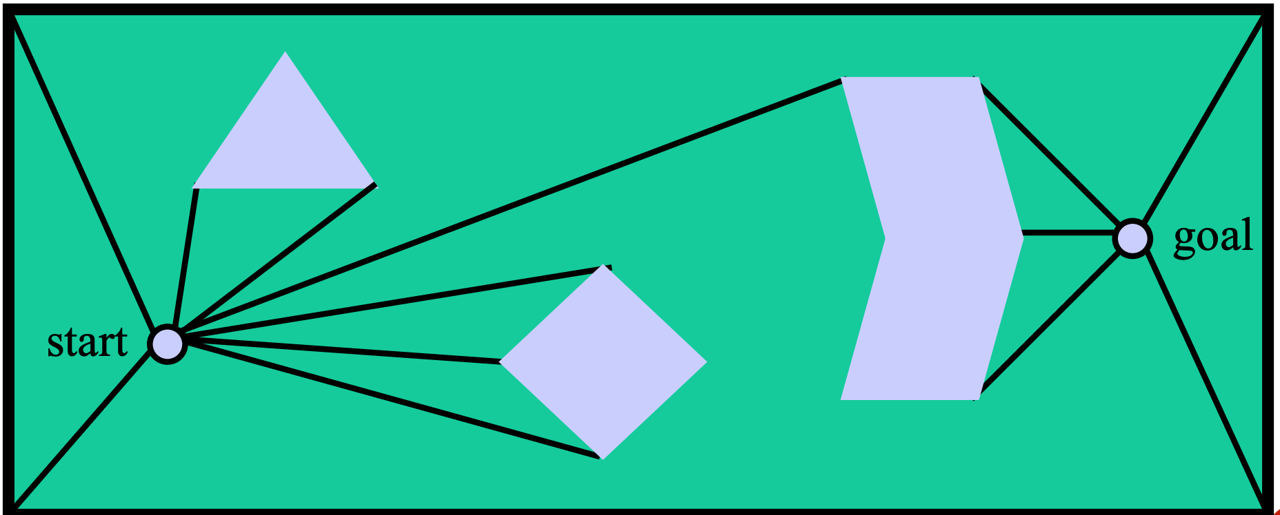
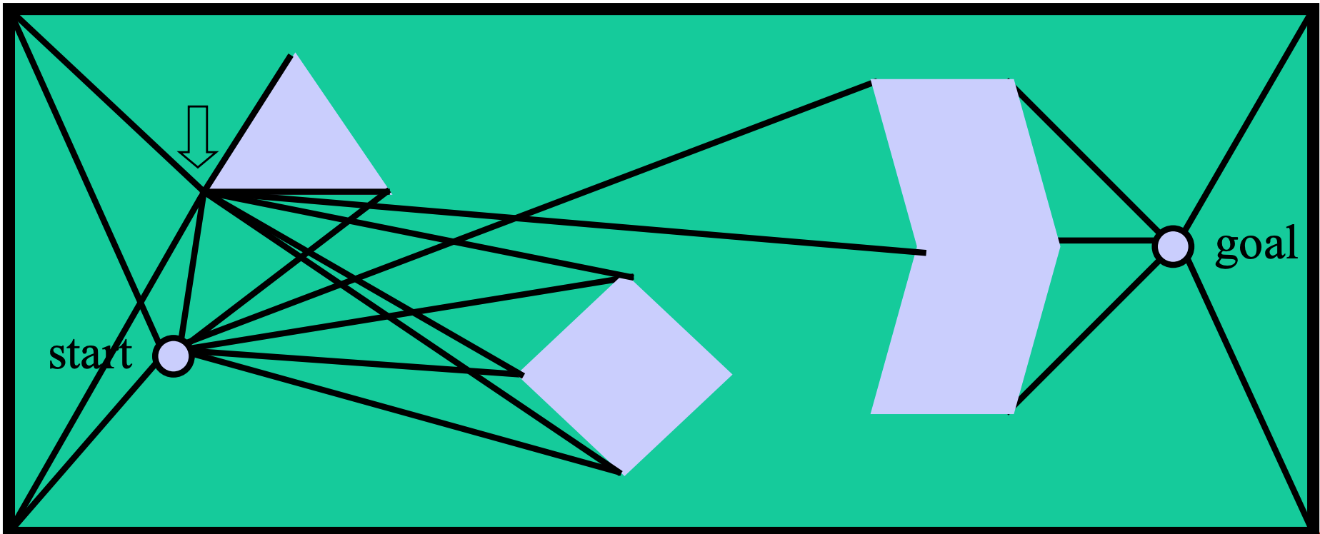
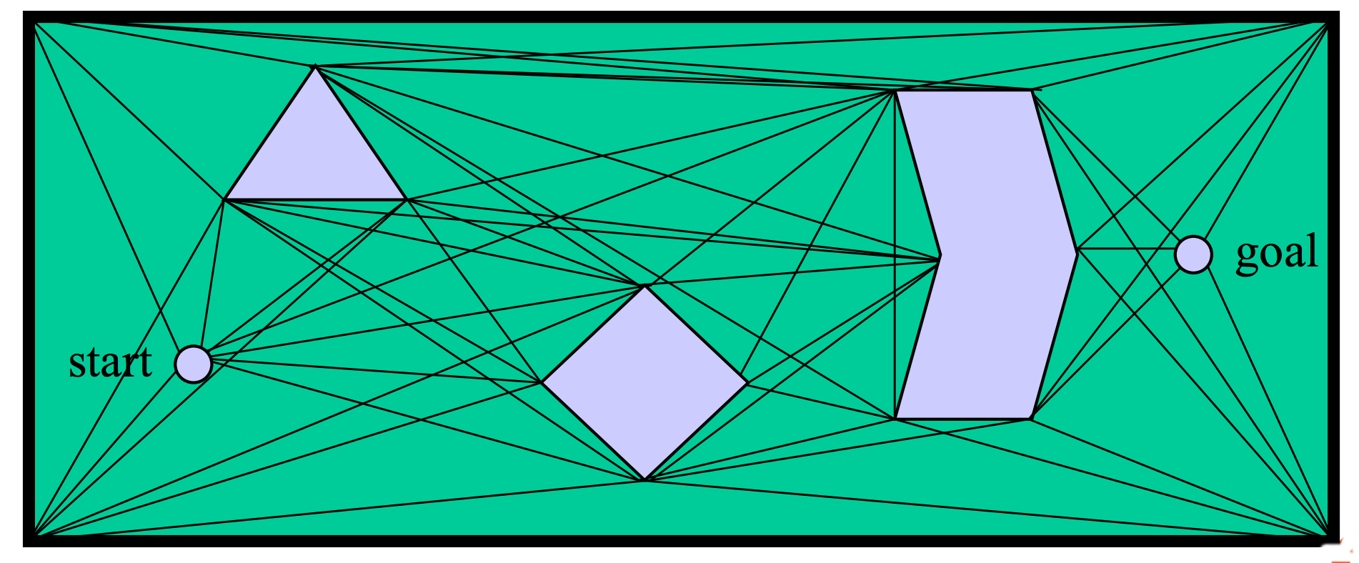
This type of representation was popular in early configuration space algorithms. It produces paths of minimal length. However, these paths aren't very safe because they skim the edges of obstacles. It's risky to get too close to obstacles. We could easily hit the obstacle if there are any errors in our model of our shape, our position, and/or the obstacle position. For most practical applications, it's better to have a somewhat longer path that is reasonably short and doesn't come too close to obstacles.
Another class of methods converts freespace into a skeleton that goes through the middle of regions, called a "roadmap". Paths via the skeleton stay far from obstacles, so they tend to be safe but perhaps overly long.
The "Generalized Voronoi Diagram" places the skeleton along curves that are equidistant from two or more obstacles. The waypoints are the places where these curves intersect.
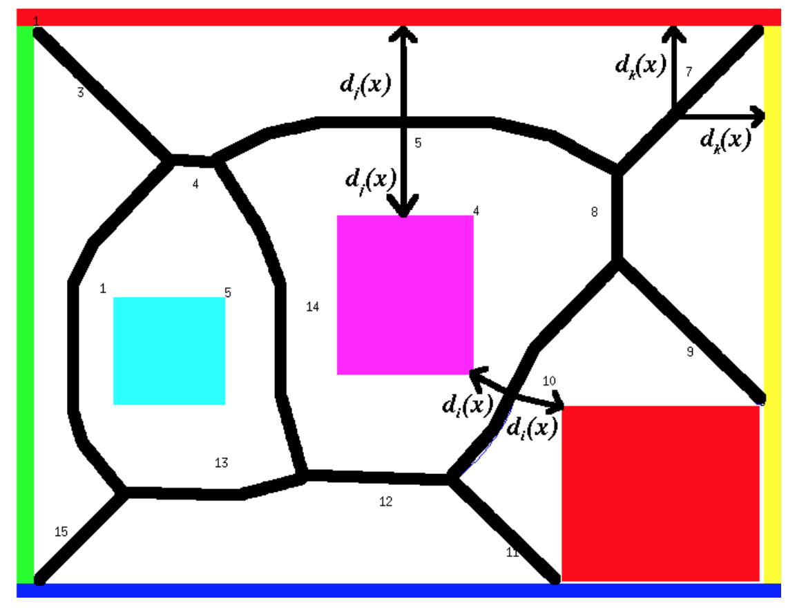 (from Howie Choset)
The cell decomposition below divides free space somewhat more arbitrarily into trapezoids aligned with the coordinate axes. Waypoints are then located in the middle of each trapezoid and the middles of its edges.
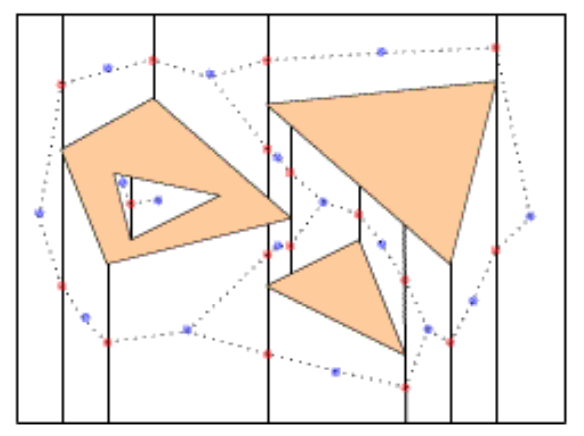 (from Philippe Cheng, MIT, 2001)
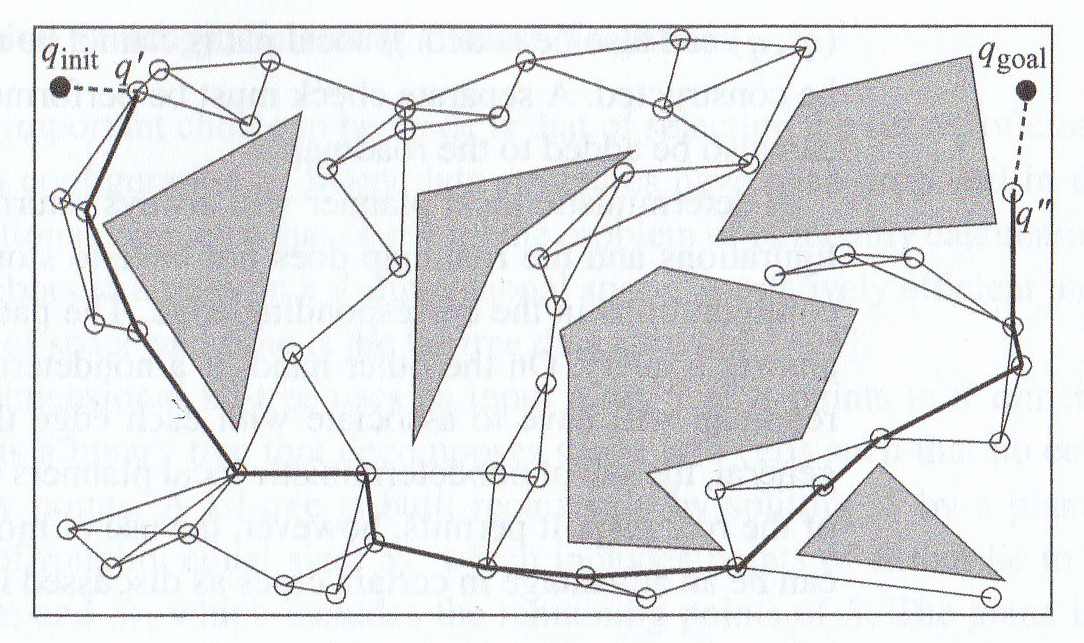
A roadmap for a configuration space is usually precomputed and then used to plan many paths, e.g. as the robot moves around its environment. The start and goal of the path will typically not be on the roadmap. So the path is constructed in three parts:
Paths assembled from roadmap edges may be longer than needed, and the edges aren't joined together smoothly. Sharp changes in orientation may be impossible for the robot to execute and/or cause excessive wear on the joints. So it is standard practice to optimize them (e.g. by smoothing the curve) in a post-processing step.
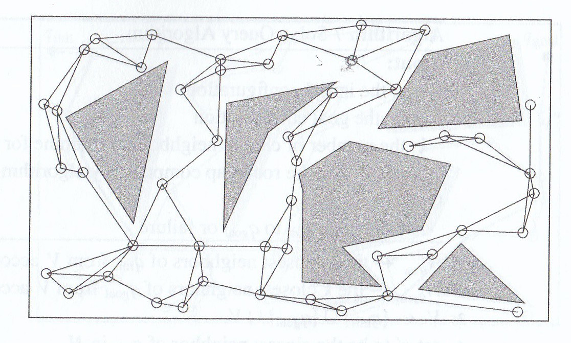
Recent algorithms create roadmaps more efficiently by sampling the configuration space without every computing the details of all the obstacles. Specifically we
There are fast algorithms for deciding whether a specific point is inside any obstacle. If waypoints are close together, there are also simple methods for connecting them, e.g. check whether the straight line between them is in free space.
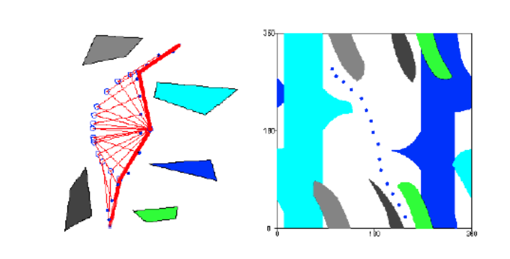
Here is a probabilistic roadmap for a simple planning problem (left) and a plan constructed using it (right).
 (
(
 (from Howie Choset book)