 Probability
 A key task in building AI systems is classification, e.g. identifying what's in a picture. We'll start by looking at statistical methods of classification, particularly Naive Bayes.
Mulberry trees have edible berries and are the dominant food of silkworms, The picture above shows a silk mill from a brief attempt (around 1834) to establish a silk industry in Northampton Massachusetts. This attempt failed despite the fact that mulberry trees grow easily in much of the US. Would you be able to tell a mulberry leaf from a birch leaf (below)? How would you even go about describing how they look different?
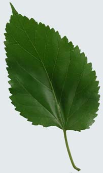
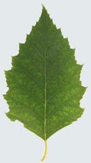
Which is mulberry and which is birch?
These pictures come Guide to Practical Plants of New England (Pesha Black and Micah Hahn, 2004). This guide includes a variety of established descrete features for identifying plants, such as
Unfortunately, both of these leaves are broad, alternate, and toothed. But they look different. (The left one is the mulberry, by the way.)
These descrete features work moderately well for plants. However, modelling categories with discrete (logic-like) features doesn't generalize well to many real-world situations.
In practice, this means that models based on yes/no answers to discrete features are incomplete and fragile A better approach is to learn models from examples, e.g. pictures, audio data, big text collections. However, this input data presents a number of challenges:
So we use probabilistic models to capture what we know, and how well we know it.
Suppose we're modelling the traffic light at University and Lincoln (two crossing streets plus a diagonal train track).
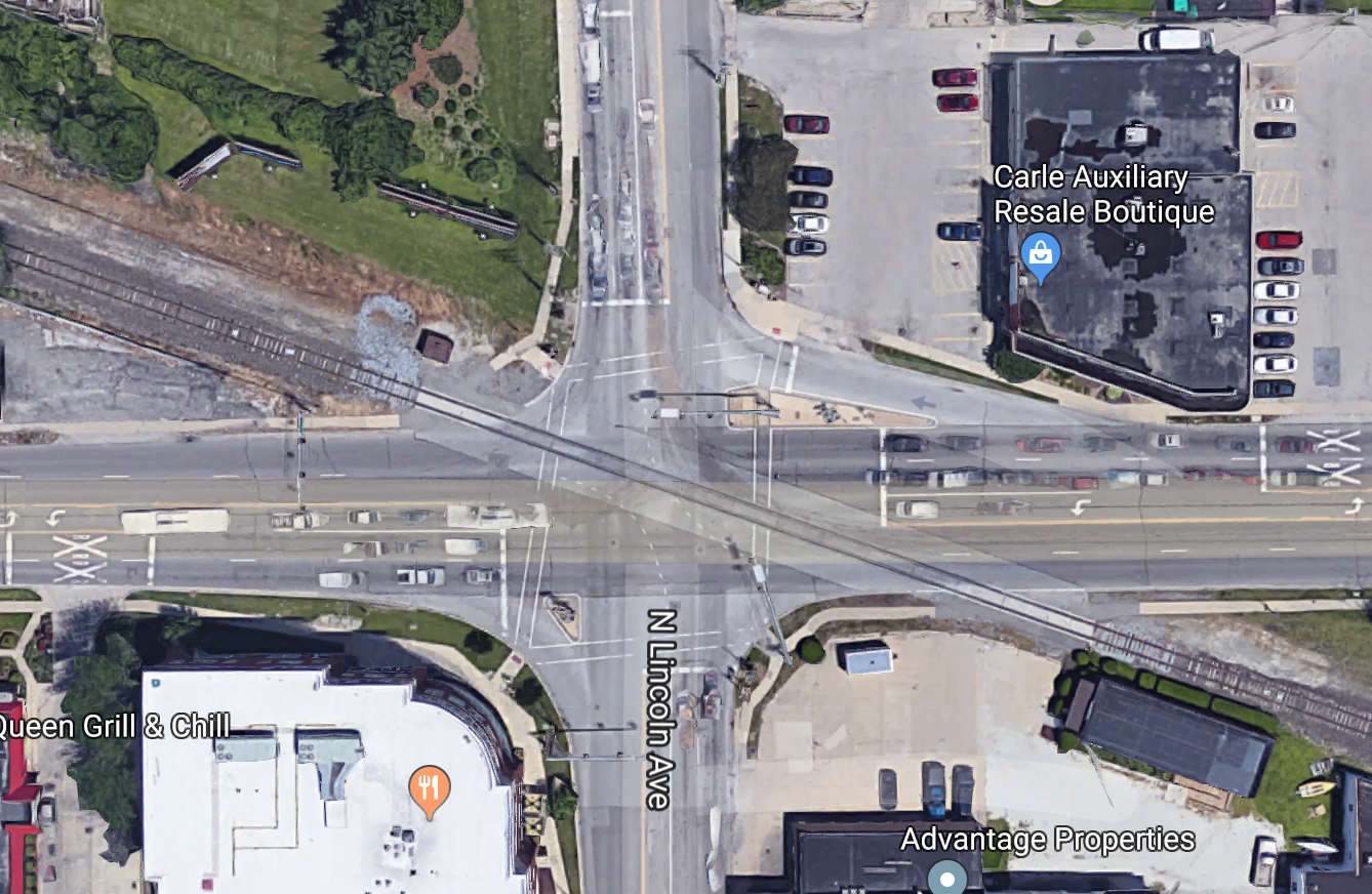
Some useful random variables might be:
| variable | domain (possible values) |
|---|---|
| time | {morning, afternoon, evening, night} |
| is-train | {yes, no} |
| traffic-light | {red, yellow, green} |
| barrier-arm | {up, down} |
Also exist continuous random variables, e.g. temperature (domain is all positive real numbers) or course-average (domain is [0-100]). We'll ignore those for now.
A state/event is represented by the values for all random variables that we care about.
P(variable = value) or P(A) where A is an event
What percentage of the time does [variable] occur with [value]? E.g. P(barrier-arm = up) = 0.95
P(X=v and Y=w) or P(X=v,Y=w)
How often do we see X=v and Y=w at the same time? E.g. P(barrier-arm=up, time=morning) would be the probability that we see a barrier arm in the up position in the morning.
P(v) or P(v,w)
The author hopes that the reader can guess what variables these values belong to. For example, in context, it may be obvious that P(up, morning) is shorthand for P(barrier-arm=up, time=morning).
Probability notation does a poor job of distinguishing variables and values. So it is very important to keep an eye on types of variable and values, as well as the general context of what an author is trying to say. A useful heuristic is that
A distribution is an assignment of probability values to all events of interest, e.g. all values for particular random variable or pair of random variables.
The key mathematical properities of a probability distribution can be derived from Kolmogorov's axioms of probability:
0 \( \le \) P(A)
P(True) = 1
P(A or B) = P(A) + P(B), if A and B are mutually exclusive events
It's easy to expand these three axioms into a more complete set of basic rules, e.g.
0 \( \le \) P(A) \( \le \) 1
P(True) = 1 and P(False) = 0
P(A or B) = P(A) + P(B) - P(A and B) [inclusion/exclusion, same as set theory]
If X has possible values p,q,r, then P(X=p or X=q or X=r) = 1.
Probabilities can be estimated from direct observation of examples (e.g. large corpus of text data). Constraints on probabilities may also come from sceientific beliefs
The assumption that anything is possible is usually made to deal with the fact that our training data is incomplete, so we need to reserve some probability for all the possible events that we haven't happened to see yet.
Here's a model of two variables for the University/Goodwin intersection:
                             E/W light
                        green       yellow   red
 N/S light   green        0          0       0.2
             yellow       0          0       0.1
             red         0.5         0.1     0.1
To be a probability distribution, the numbers must add up to 1 (which they do in this example).
Most model-builders assume that probabilities aren't actually zero. That is, unobserved events do occur but they just happen so infrequently that we haven't yet observed one. So a more realistic model might be
                             E/W light
                        green         yellow     red
 N/S light   green        e            e         0.2-f
             yellow       e            e         0.1-f
             red         0.5-f       0.1-f       0.1-f
To make this a proper probability distribution, we need to set
f=(4/5)e so all the values add up to 1.
Suppose we are given a joint distribution like the one above, but we
want to pay attention to only one variable. To get its distribution,
we sum probabilities across all values of the other variable.
So the marginal distribution of the N/S light is
To write this in formal notation
suppose Y has values \( y_1 ... y_n \). Then
we compute the marginal probability P(X=x) using the formula
\( P(X=x) = \sum_{k=1}^n P(x,y_k) \).
Suppose we know that the N/S light is red, what are the probabilities for the
E/W light? Let's just extract that line of our joint distribution.
The notation for a conditional probability looks like P(event | context).
If we just pull numbers out of this row of our joint distribution, we
get a distribution that looks like this:
Oops, these three probabilities don't sum to 1. So this isn't a legit probability
distribution (see Kolmogorov's Axioms above). To make them sum to 1,
divide each one by the sum they currently have (which is 0.7).
So, in the context where N/S is red, we have this distribution:
Conditional probability models how frequently we see each variable value in some context
(e.g. how often is the barrier-arm down if it's nighttime).
The conditional probability of A in a context C is defined to be
Many other useful formulas can be derived from this definition plus
the basic formulas given above. In particular, we can transform
this definition into
These formulas extend to multiple inputs like this:
Two events A and B are independent iff
It's equivalent to show that this equation is equivalent to
each of the following equations:
Exercise for the reader: why are these three equations all equivalent? Hint: use
definition of conditional probability.
Figure this out for yourself, because it will help you become familiar with the
definitions.
We have two types of bike (veoride and standard). Veorides are
mostly teal (with a few exceptions), but other (privately owned)
bikes rarely are.
Joint distribution for these two variables
For this toy example, we can fill out the joint distribution table.
However, when we have more variables (typical of AI problems), this isn't
practical. The joint distribution contains
Remember that
P(A | C) is the probability of A in a context where C is true.
For example, the probability of a bike being teal increases dramatically
if we happen to know that it's a veobike.
The formal definition:of conditional probability is
Let's write this in the equivalent form P(A,C) = P(C) * P(A | C).
Flipping the roles of A and C (seems like middle school but just keep reading):
P(A,C) and P(C,A) are the same quantity. (AND is commutative.) So we have
So
So we have Bayes rule
Here's how to think about the pieces of this formula
The normalization doesn't have a proper name because we'll typically
organize our computation so as to eliminate it. Or, sometimes, we won't
be able to measure it directly, so the number will be set at
whatever is required to make all the probability values add up to 1.
Example: we see a teal bike. What is the chance that it's a veoride?
We know
So we can calculate
In non-toy examples, it will be easier to get estimates for
P(evidence | cause) than direct estimates for P(cause | evidence).
P(evidence | cause) tends to be stable, because it is due to some
underlying mechanism. In this example, veoride likes teal and
regular bike owners don't. In a disease scenario, we might be
looking at the tendency of measles to cause spots, which is due to a
property of the virus that is fairly stable over time.
P(cause | evidence) is less stable, because it depends on the set
of possible causes and how common they are right now.
For example, suppose that a critical brake problem is discovered and
Veoride suddenly has to pull bikes into the shop for repairs. So then
only 2% of the bikes are veorides.
Then we might have the following joint
distribution. Now a teal bike is more likely to be
standard rather than veoride.
Dividing P(cause | evidence) into P(evidence | cause) and P(cause)
allows us to easily adjust for changes in P(cause).
Recall Bayes Rule:
Example: We have two underlying types of bikes: veoride and standard.
We observe a teal bike. What type should we guess that it is?
"Maximum a posteriori" (MAP) estimate chooses the type with the
highest posterior probability:
Suppose that type X comes from a set of types T. Then MAP chooses
The argmax operator iterates through a series of values for the dummy variable (X in
this case). When it determines the maximum value for the quantity (P(X | evidence)
in this example), it returns the value for X that produced that maximum value.
Completing our example, we compute two posterior probabilities:
The first probability is bigger, so we guess that it's a veoride. Notice that
these two numbers add up to 1, as probabilities should.
P(evidence) can usually be factored out of these equations, because
we are only trying to determine the relative probabilities. For the
MAP estimate, in fact, we are only trying to find the largest
probability. In our equation
P(evidence) is the same for all the causes we are considering. Said another
way, P(evidence) is the probability that we would see this evidence if we
did a lot of observations. But our current situation is that we've actually
seen this particular evidence and we don't really care if we're analyzing
a common or unusual situation.
So Bayesian estimation often works with the equation
where we know (but may not always say) that the normalizing constant is
the same across various such quantities.
Specifically, for our example
P(teal) is the same in both quantities. So we can remove it, giving us
So veoride is the MAP choice, and we never needed to know P(teal). Notice
that the two numbers (0.19 and 0.02) don't add up to 1. So they aren't
probabilities, even though their ratio is the ratio of the probabilities
we're interested in.
As we saw above, our joint probabilities depend on the relative
frequencies of the two underlying causes/types. Our MAP estimate
reflects this by including the prior probability.
If we know that all causes are equally likely,
we can set all P(cause) to the same value
for all causes. In that case, we have
So we can pick the cause that maximizes P(evidence | cause).
This is called the "Maximum Likelihood Estimate" (MLE).
The MLE estimate
can be very inaccurate if the prior probabilities of different
causes are very different.
On the other hand, it can be a sensible choice if we have
poor information about the prior probabilities.
                             E/W light                marginals
                        green       yellow   red
 N/S light   green        0          0       0.2        0.2
             yellow       0          0       0.1        0.1
             red         0.5         0.1     0.1        0.7
-------------------------------------------------
marginals                0.5         0.1     0.4
P(green) = 0.2
P(yellow) = 0.1
P(red) = 0.7
Conditional probabilities
                             E/W light
                        green       yellow      red
 N/S light   red         0.5         0.1         0.1
P(E/W=green | N/S = red) = 0.5
P(E/W=yellow | N/S = red) = 0.1
P(E/W=red | N/S = red) = 0.1
P(E/W=green) = 0.5/0.7 = 5/7
P(E/W=yellow) = 0.1/0.7 = 1/7
P(E/W=red) = 0.1/0.7 = 1/7
Conditional probability equations
P(A | C) = P(A,C)/P(C)
P(A,C) = P(C) * P(A | C)
P(A,C) = P(A) * P(C | A)
P(A,B,C) = P(A) * P(B | A) * P(C | A,B)
Independence
P(A,B) = P(A) * P(B)
P(A | B) = P(A)
P(B | A) = P(B)
Bikes
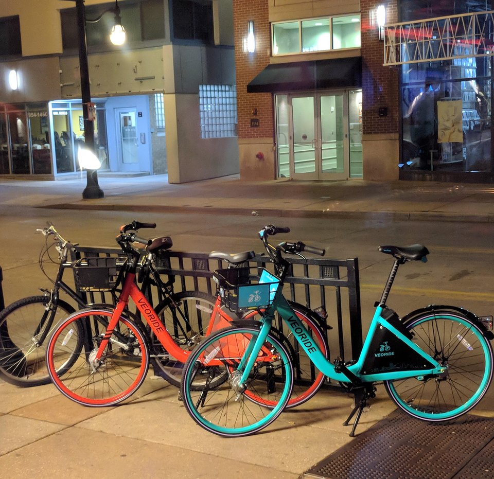 Red and teal veoride bikes from
/u/civicsquid reddit post
Red and teal veoride bikes from
/u/civicsquid reddit post
Example: campus bikes
                 veoride        standard     |
    teal            0.19          0.02       |   0.21
    red             0.01          0.78       |   0.79
                 ----------------------------
                    0.20          0.80
The estimation is the more important problem because we usually
have only limited amounts of data, esp. clean annotated data. Many
value combinations won't be observed simply because we haven't seen
enough examples.
Bayes Rule
P(teal) = 0.21
P(teal | veoride) = 0.95 (19/20)
P(A | C) = P(A,C)/P(C)
equivalently P(C,A) = P(A) * P(C | A)
P(A) * P(C | A) = P(A,C) = P(C) * P(A | C)
P(A) * P(C | A) = P(C) * P(A | C)
P(C | A) = P(A | C) * P(C) / P(A)
       P(cause | evidence) =  P(evidence | cause) *  P(cause) / P(evidence)

         posterior            likelihood             prior     normalization
P(teal | veoride) = 0.95 [likelihood]
P(veoride) = 0.20 [prior]
P(teal) = 0.21 [normalization]
P(veoride | teal) = 0.95 x 0.2 / 0.21 = 0.19/0.21 = 0.905
Why will this be useful?
                 veoride        standard     |
    teal            0.019          0.025     |   0.044
    red             0.001          0.955     |   0.956
                 ----------------------------
                    0.02           0.98
The MAP estimate
       P(cause | evidence) =  P(evidence | cause) *  P(cause) / P(evidence)

       posterior            likelihood             prior     normalization
pick the type X such that P(X | evidence) is highest
\(\arg\!\max_{X \in T} P(X | \text{evidence}) \)
P(veoride | teal) = 0.905
P(standard | teal) = 0.095
Ignoring the normalizing factor
P(cause | evidence) = P(evidence | cause) * P(cause) / P(evidence)
P(cause | evidence) \( \propto \) P(evidence | cause) * P(cause)
P(veoride | teal) = P(teal | veoride) * P(veoride) / P(teal)
P(standard | teal) = P(teal | standard) * P(standard) / P(teal)
P(veoride | teal) \( \propto \) P(teal | veoride) * P(veoride) = 0.95 * 0.2 = 0.19
P(standard | teal)
\( \propto \) P(teal | standard) * P(standard) = 0.025 * 0.8 = 0.02
The MLE estimate
P(cause | evidence) \( \propto \) P(evidence | cause)