So far, we've seen some systems containing more than one classifier unit, but each unit was always directly connected to the inputs and an output. When people say "neural net," they usually mean a design with more than layer of units, including "hidden" units which aren't directly connected to the output. Early neural nets tended to have at most a couple hidden layers (as in the picture below). Modern designs typically use many layers.
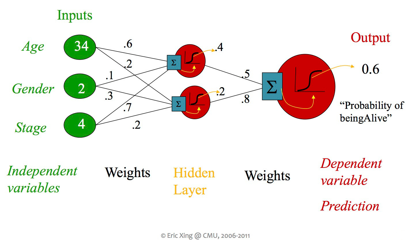
from Eric Xing via Matt Gormley
A single unit in a neural net can look like any of the linear classifiers we've seen previously. Moreover, different layers within a neural net design may use types of units (e.g. different activation functions). However, modern neural nets typically use entirely differentiable functions, so that gradient descent can be used to tune the weights.
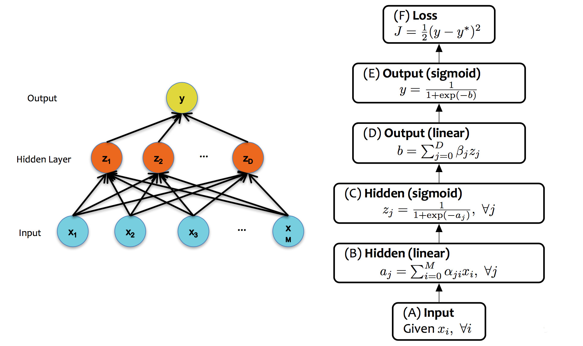
from Matt Gormley
Notice two things about this design. First, each layer has its own activation function, but there is only one loss function, at the very end. Second, the activation functions are non-linear. If we had linear activation functions, we could squash the whole network down into one linear function, so we'd be back to having only linear classification boundaries.
The core ideas in neural networks go back decades. Some of their recent success is due to better understanding of design and/or theory. But perhaps the biggest reasons have to do with better computer hardware and better library support for the annoying mechanical parts of the computation.
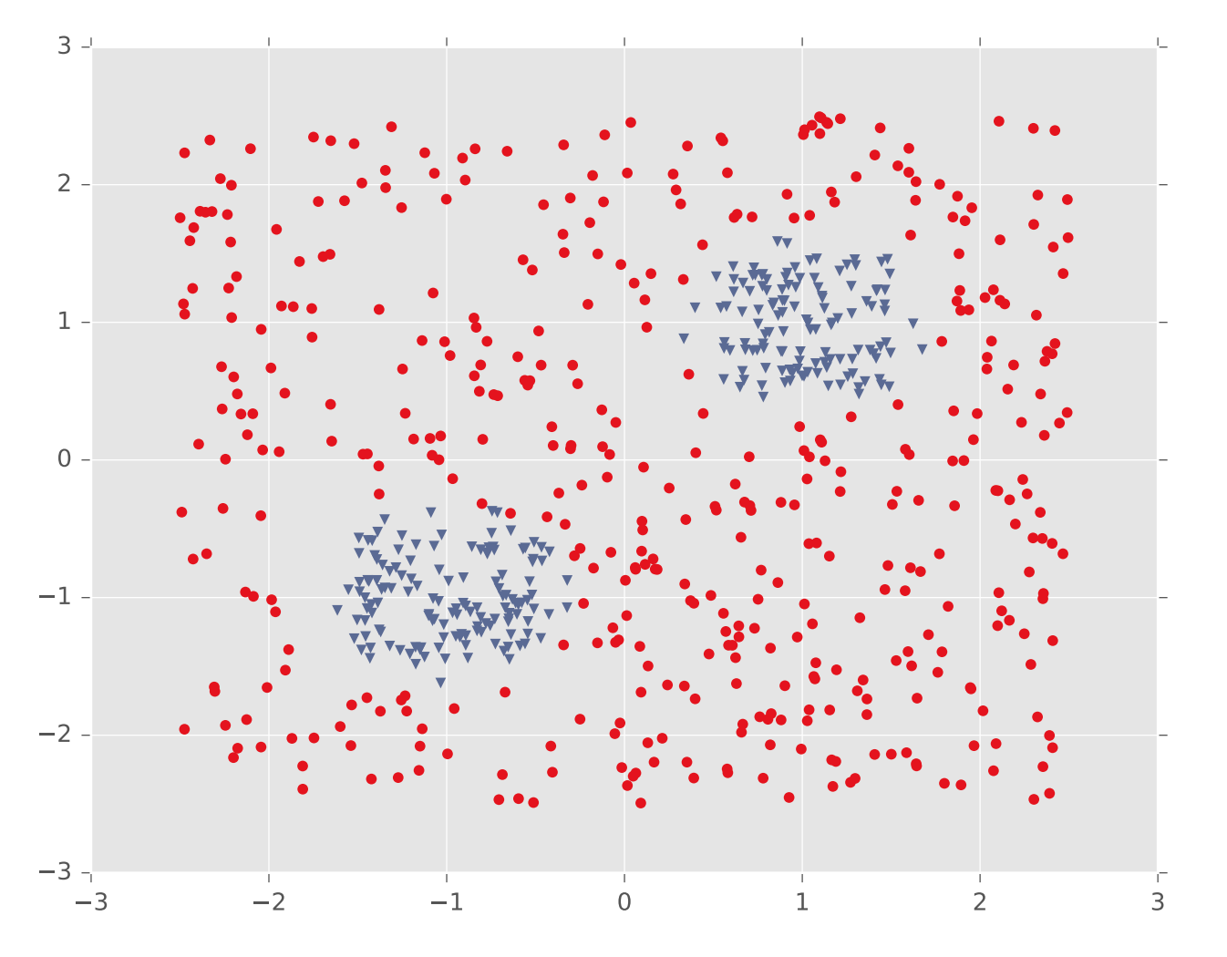
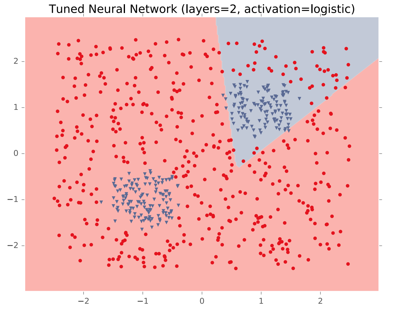
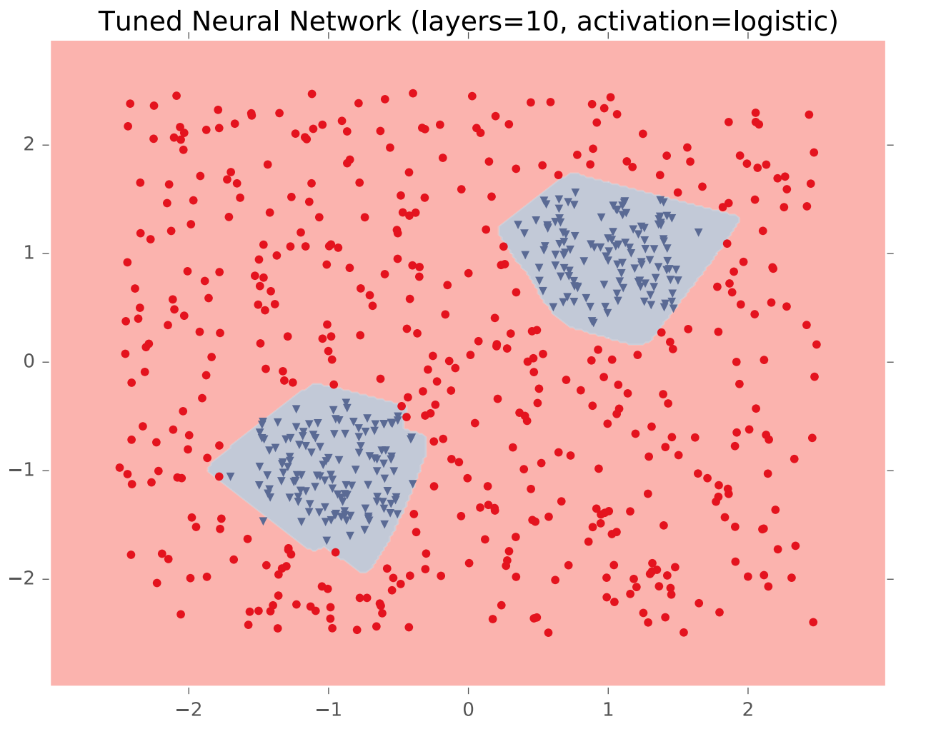
In theory, a single hidden layer is sufficient to approximate any continuous function, assuming you have enough hidden units. However, shallow networks may require very large numbers of hidden units. Deeper neural nets seem to be easier to design and train. Here's an example (from Matt Gormley) of a class boundary with a somewhat complex shape. K-nearest neighbor does a good job of approximating it (but is inefficient in higher dimensions).
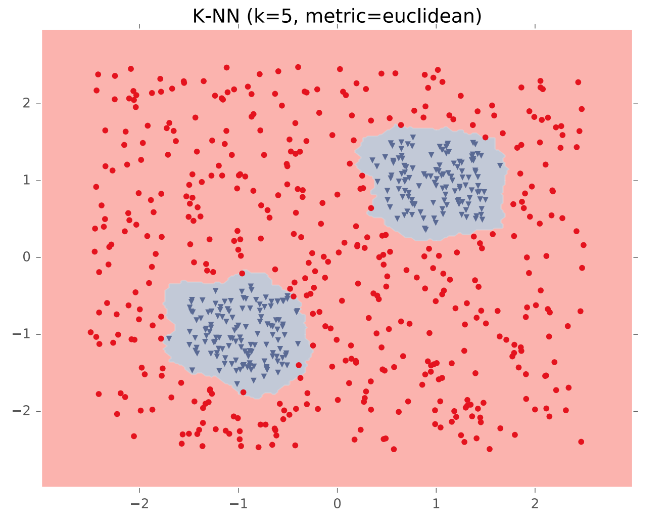
A two-layer network gives us a poor approximation (left), but a ten-layer network does a good job (right). Notice that our final network model is compact: proportional to the number of weights int the network. The size of k-nearest neighbor model grows with the number of training samples.
In image processing applications, deep networks normally emulate the layers of processing found in previous human-designed classifiers. So each layer transforms the input so as to make it more sophisticated ("high level"), compacts large inputs (e.g. huge pictures) into a more manageable set of features, etc. The picture below shows a face recognizer in which the bottom units detect edges, later units detect small pieces of the face (e.g. eyes), and the last level (before the output) finds faces.
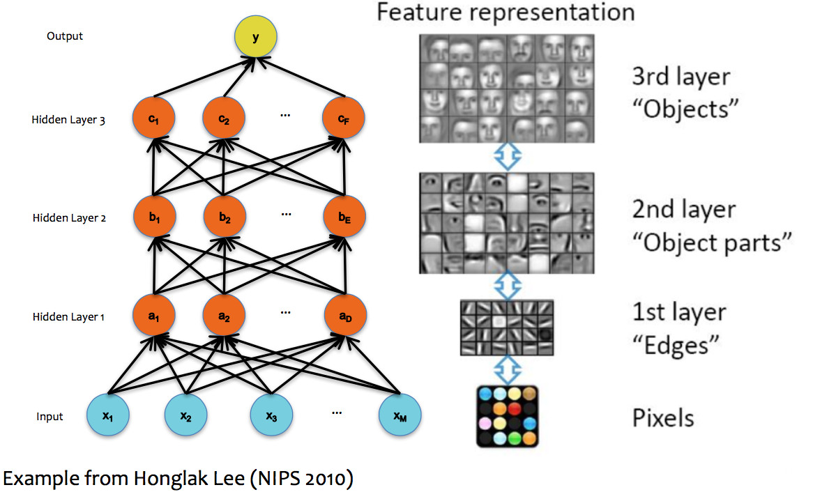
(from Matt Gormley)
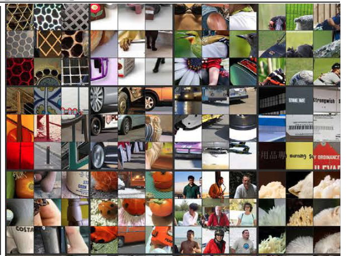
Here are layers 1, 3, and 5 from a neural net trained on ImageNet (from M. Zeiler and R. Fergus Visualizing and Understanding Convolutional Networks).
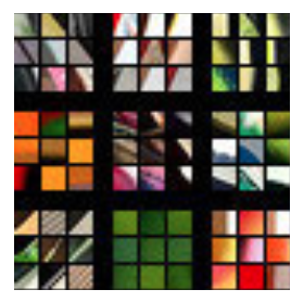
from Matt Gormley
Neural nets are trained in much the same way as individual classifiers. That is, we initialize the weights, then sweep through the input data multiple types updating the weights. When we see a training pair, we updated the weights, moving each weight \(w_i\) in the direction that decreases the loss (J):
\( w_i = w_i - \alpha * \frac{\partial J}{\partial w_i} \)
Notice that the loss is available at the output end of the network, but the weight \(w_i\) might be in an early layer. So the two are related by a chain of composed functions, often a long chain of functions. We have to compute the derivative of this composition.
Remember the chain rule from calculus. If \(h(x) = f(g(x)) \), the chain rule says that \(h'(x) = f'(g(x))\cdot g'(x) \). In other words, to compute \(h'(x) \), we'll need the derivatives of the two individual functions, plus the value of of them applied to the input.
Let's write out the same thing in Liebniz notation, with some explicit variables for the intermediate results:
This version of the chain rule now looks very simple: it's just a product. However, to evaluate this function at an input value x, we need to remember that it depends implicitly on the equations defining y in terms of x, and z in terms of y. Let's use the term "forward values" for values like y and z.
We can now see that the derivative for a whole composed chain of functions is, essentially, the product of the derivatives for the individual functions. So, for a weight w at some level of the network, we can assemble the value for \( \frac{\partial J}{\partial w} \) using
Now, suppose we have a training pair (\(\vec{x}, y)\). (That is, y is the correct class for \(\vec{x}\).) Updating the neural net weights happens as follows:
Notice that all these quantities are evaluated at the input value \(\vec{x}\).
The diagram below shows the forward and backward values for our example network:
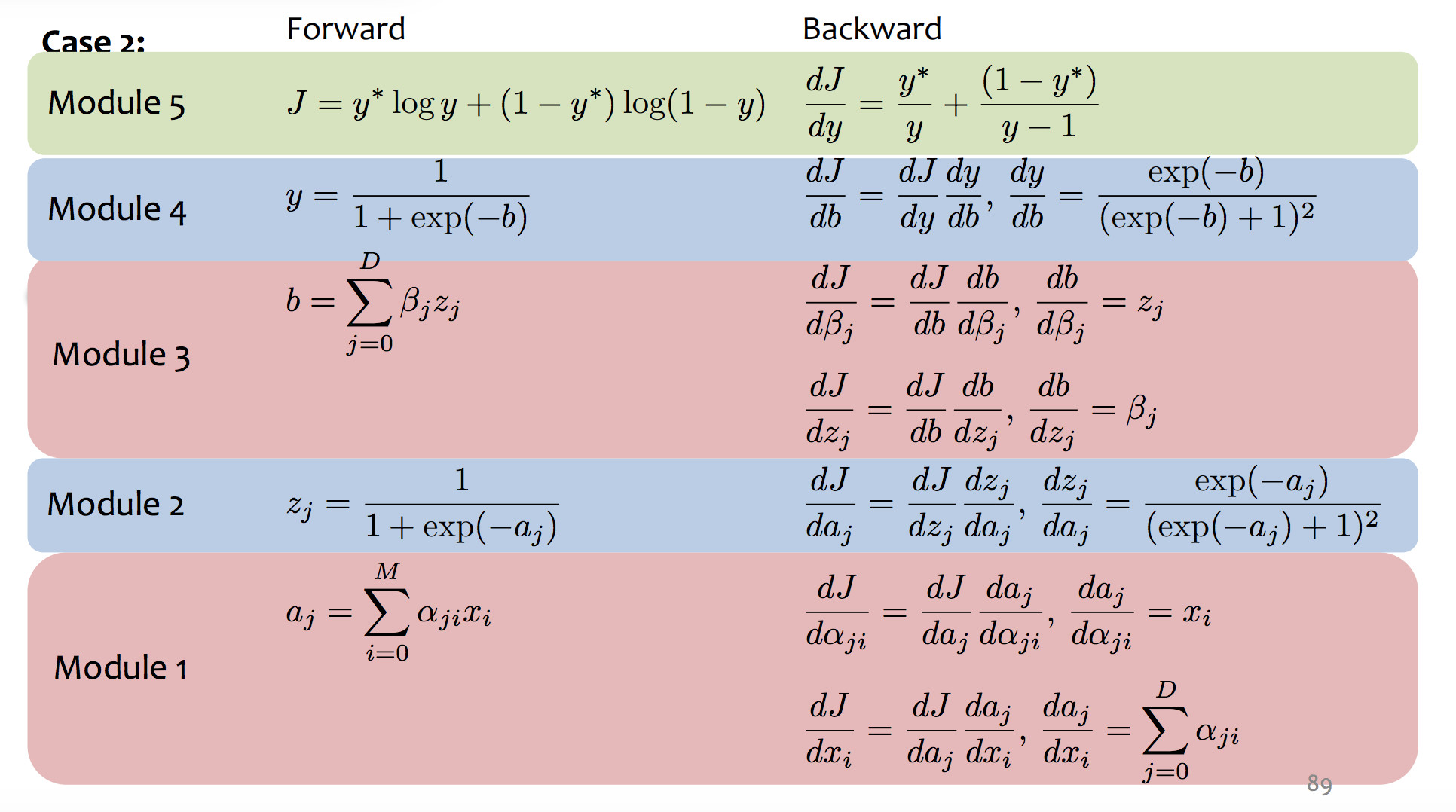
(from Matt Gormley)
Backpropagation is essentially a mechanical exercise in applying the chain rule repeatedly. Humans make mistakes, and direct manual coding will have bugs. So, as you might expect, computers have taken over most of the work as they for (say) register allocation. Read the very tiny example in Jurafsky and Martin (7.4.3 and 7.4.4) to get a sense of the process, but then assume you'll use TensorFlow or PyTorch to make this happen for a real network.
Unfortunately, training neural nets is somewhat of a black art because the process isn't entirely stable. Three issues are prominent:
Perceptron training works fine with all weights initialized to zero. This won't work in a neural net, because each layer typically has many neurons connected in parallel. We'd like parallel units to look for complementary features but the naive training algorithm will cause them to have identical behavior. At that point, we might as well economize by just having one unit. Two approaches to symmetry breaking:
One specific proposal for randomization is dropout: Within the network, each unit pays attention to training data only with probability p. On other training inputs, it stops listening and starts reading its email or something. The units that aren't asleep have to classify that input on their own. This can help prevent overfitting.
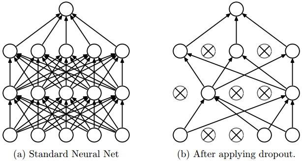
from Srivastava et al.
Neural nets infamously tend to tune themselves to peculiarities of the dataset. This kind of overfitting will make them less able to deal with similar real-world data. The dropout technique will reduce this problem. Another method is "data augmentation".
Data augmentation tackles the fact that training data is always very sparse, but we have additional domain knowledge that can help fill in the gaps. We can make more training examples by perturbing existing ones in ways that shouldn't (ideally) change the network's output. For example, if you have one picture of a cat, make more by translating or rotating the cat. See this paper by Taylor and Nitschke.
Another approach to reducing overfitting is "regularization." Suppose that our set of training data is T. Then, rather than minimizing loss(model,T), we minimize
loss(model,T) + \(\lambda\) * complexity(model)
The right way to measure model complexity depends somewhat on the task. A simple method for a linear classifier would be \(\sum_i (w_i)^2 \), where the \(w_i\) are the classifier's weights. Recall that squaring makes the L2 norm sensitive to outlier (aka wrong) input values. In this case, this behavior is a feature: this measure of model complexity will pay strong attention to unusually large weights and make the classifier less likely to use them. Linguistic methods based on "minimumum description length" are using a variant of the same idea.
\(\lambda \) is a constant that balances the desire to fit the data with the desire to produce a simple model. This is yet another parameter that would need to be tuned experimentally using our development data. The picture below illustrates how the output of a neural net classifier becomes simpler as \(\lambda \) is increased. (The neural net in this example is more complex, with hidden units.)
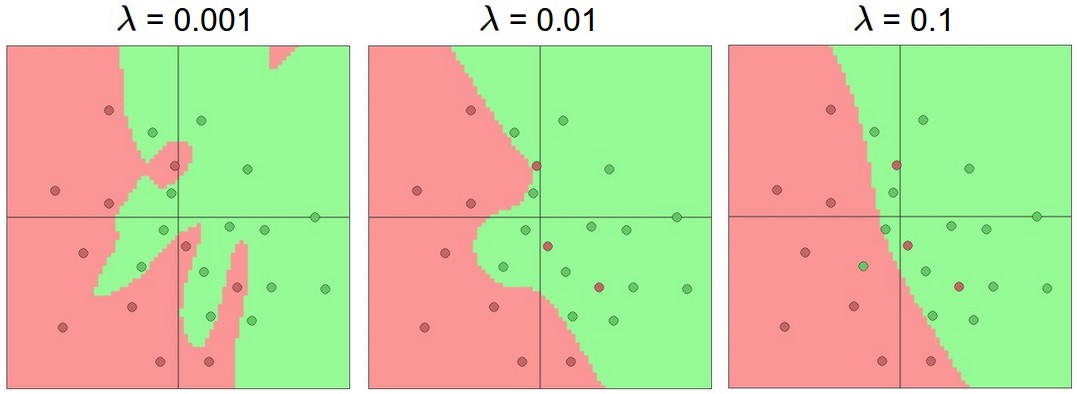
from
Andrej Karpathy course notes
In order for training to work right, gradients computed during backprojection need to stay in a sensible range of sizes. A sigmoid activation function only works well when output numbers tend to stay in the middle area that has a significant slope.
The underflow/overflow issues happen because numbers that are somewhat too small/large tend to become smaller/larger.
Several approaches to mitigating this problem, none of which looks (to me) like a solid, complete solution.
To train the neural net, we make many passes through the training data. An "epoch" is one pass through all the training data.
Processing the training data pair by pair is slow. Normally we group the training pairs into small sets ("batches" or "mini-batches"). For each set, we compute the gradients for each pair, average all the gradients, and do one update to the neural net's weights. A single epoch of training will typically require processing many batches of training data. Most of the bookkeeping details are handled by special "dataloader" software.
Convolutional neural nets are a specialized architecture designed to work well on image data (also apparently used somewhat for speech data). Images have two distinctive properties:
We'd like to be able to do some processing at high-resolution, to pick out features such as written text. But other objects (notably faces) can be recognized with only poor resolution. So we'd like to use different amounts of resolution at different stages of processing.
The large size of each layer makes it infeasible to connect units to every unit in the previous layer. Full interconnection can be done for artificially small (e.g. 32x32) input images. For larger images, this will create too many weights to train effectively with available training data. For physical networks (e.g. the human brain), there is also a direct hardware cost for each connection.
In a CNN, each unit reads input only from a local region of the preceding layer:
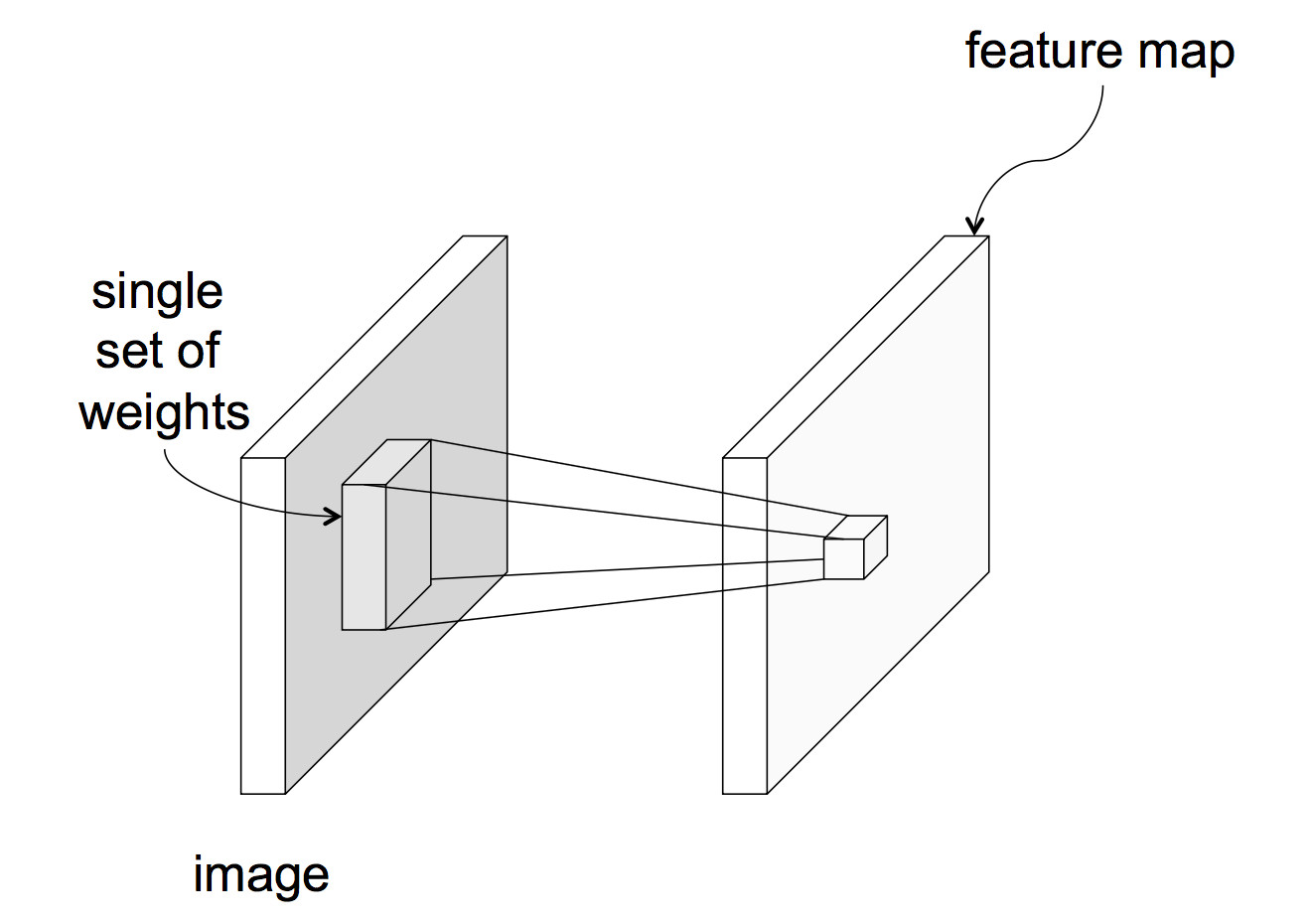
from Lana Lazebnik Fall 2017
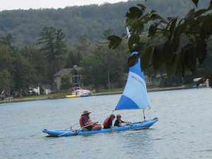
This means that each unit computes a weighted sum of the values in that local region. In signal processing, this is known as "convolution" and the set of weights is known as a "mask." For example, the following mask will locate sharp edges in the image.
              0   -4    0
             -4   16   -4
              0   -4    0
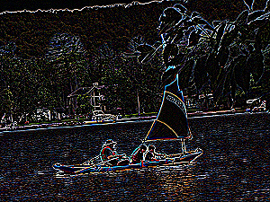
The following mask detects horizontal edges but not vertical ones.
               2    4     8    4    2
               0    0     0    0    0
              -2   -4    -8   -4   -2
These examples were made with gimp (select filters, then generic).
Normally, all units in the same layer would share a common set of weights and bias terms, called "parameter sharing". This reduces the number of parameters we need to train. However, parameter sharing may worsen performance if different regions in the input images are expected to have different properties, e.g. the object of interest is always centered. (This might be true in a security application where people were coming through a door.) So there are also neural nets in which separate parameters are trained for each unit in a convolutional layer.
The above picture assumes that each layer of the network has only one value at each (x,y) position. This is typically not the case. An input image often has three values (red, green, blue) at each pixel. Going from the input to the first hidden layer, one might imagine that a number of different convolution masks would be useful to apply, each picking out a different type of feature. So, in reality, each network layer has a significant thickness, i.e. a number of different values at each (x,y) location.
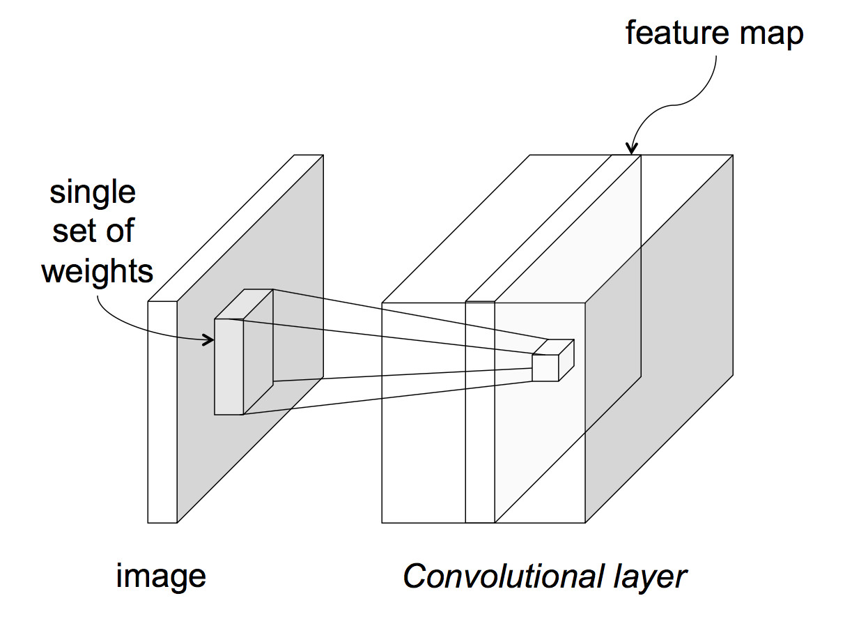
from Lana Lazebnik Fall 2017
Click on the image below to see an animation from Andrej Karpathy shows how one layer of processing might work:
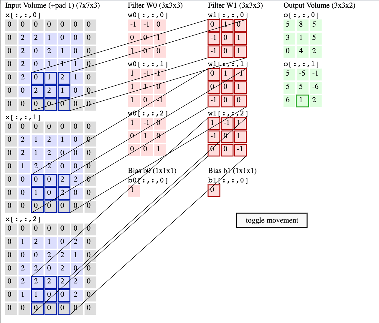
In this example, each unit is producing values only at every third input location. So the output layer is a 3x3 image, with has two values at each (x,y) position.
Two useful bits of jargon:
If we're processing color images, the initial input would have depth 3. But the depth might get significantly larger if we are extracting several different types of features, e.g. edges in a variety of orientations.
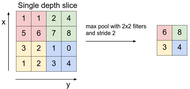
A third type of neural net layer reduces the size of the data, by producting an output value only for every kth input value in each dimension. This is called a "pooling" layer. The output values may be either selected input values, or the average over a group of inputs, or the maximum over a group of inputs.
 from
Andrej Karpathy
from
Andrej Karpathy
This kind of reduction in size ("downsampling") is especially sensible when data values are changing only slowly across the image. For example, color often changes very slowly except at object boundaries, and the human visual system represents color at a much lower resolution than brightness.
A pooling layer that chooses the maximum value can be very useful when we wish to detect high-resolution features but don't care about their precise location. E.g. perhaps we want to report that we found a corner, together with its approximate location.
A complete CNN typically contains three types of layers
Convolutional layers would typically be found in the early parts of the network, where we're looking at large amounts of image data. Fully-connected layers would make final decisions towards the end of the process, when we've reduced the image data to a smallish set of high-level features.
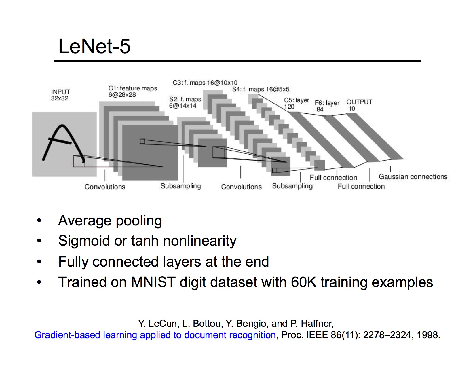
The specific network in this picture is from work by Yann LeCun and colleagues in 1998, when neural nets were just starting to be able to do something useful. Its input is very small, black and white, pictures of handwritten digits. The original application was reading zip codes for the post office.
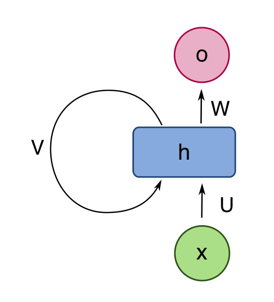
Recurrent neural nets (RNNs) are neural nets that have connections that loop back from a layer to the same layer. The RNN shown below has a single hidden layer. We can think of the self-connected layer as containing multiple processing units, similar to the hidden layer of a normal neural network. The intent of the feedback loop in the picture is that each unit is connected to all the other units in the layer.
 from Wikipedia
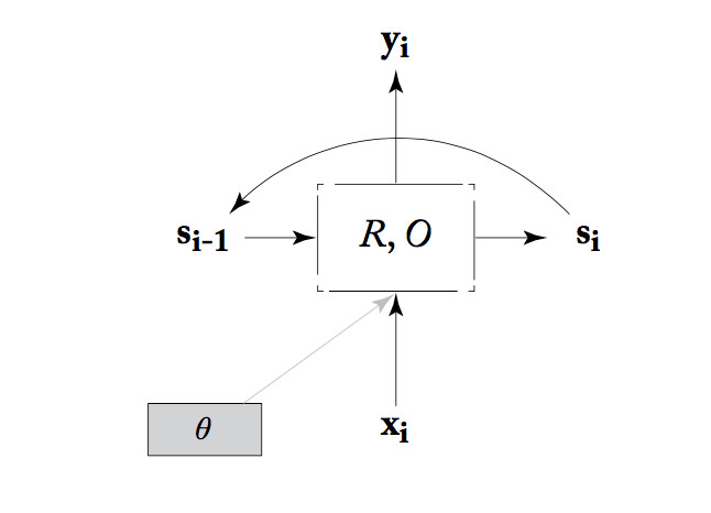
Alternatively, we can think of an RNN as a state machine. That is, we think of the values from all the units in the layer as bundled up into a state vector, \(s_i \) in the picture below. At each timestep, the RNN reads an input vector and the current state. It produces an output vector and a new state, using a state transition function (R), an output function (O), and some tunable parameters \(\theta\).
 from Yoav Goldberg
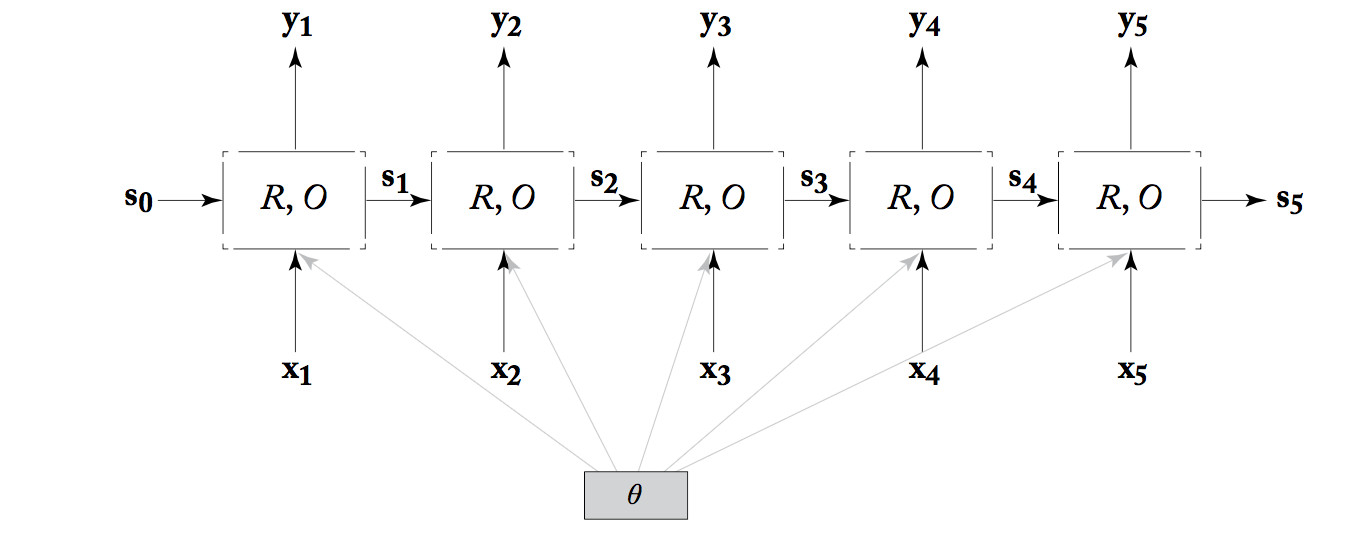
To see how computation proceeds and, more importantly, how training works, we unroll the RNN. That is, we make a clone of the RNN for each timestep, creating the diagram below. Notice that all copies of the unit share the same parameter values.
 from Yoav Goldberg
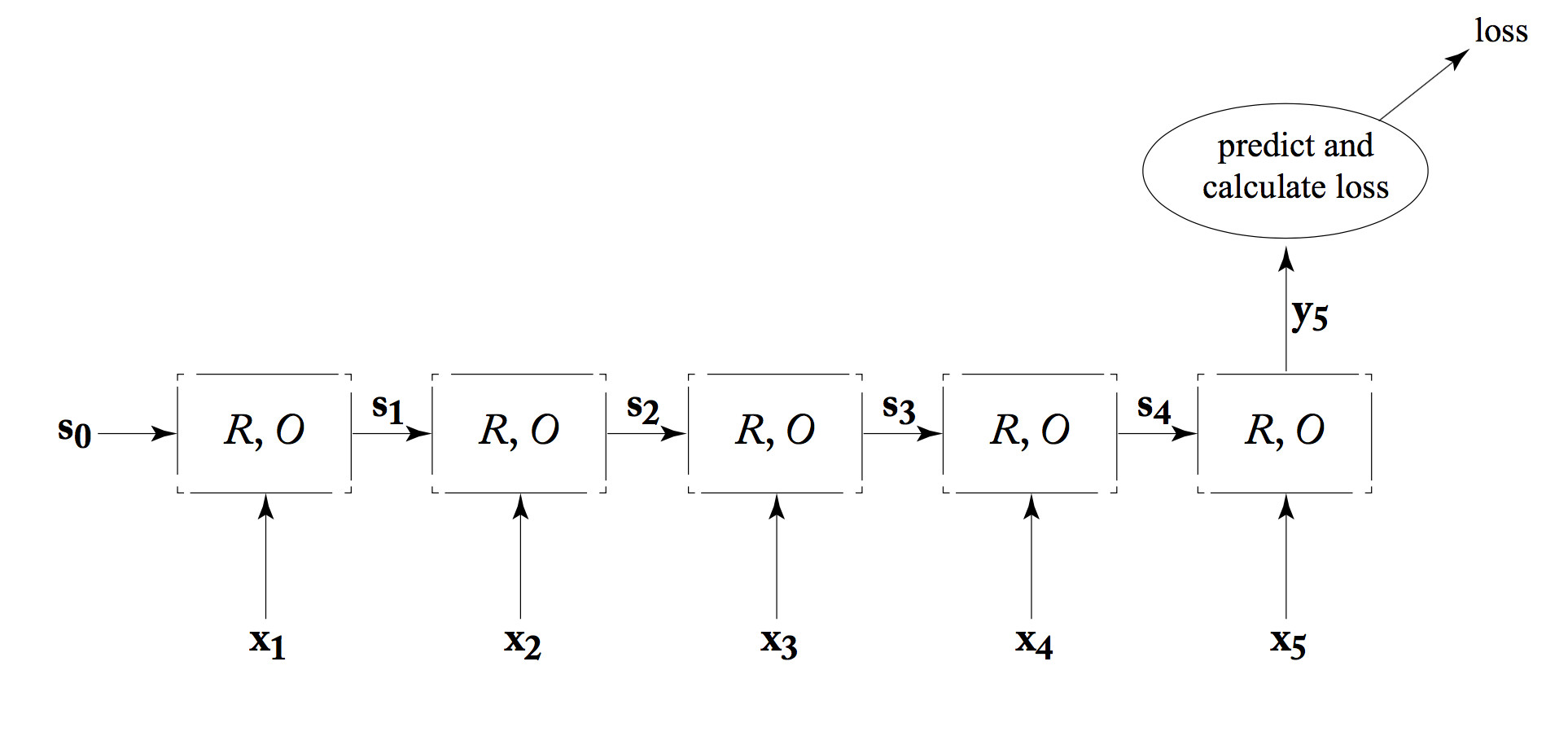
An RNN can be used as a classifier. That is, the system using the RNN only cares about the output from the last timestep, as shown below. In an NLP system, the final output value may actually be complex, e.g. a summary of an entire sentence. Either way, the final output value is fed into a later processing that provides feedback about its performance (the loss value).
 from Yoav Goldberg
This kind of RNN can be trained in much the same way as a standard ("feedforward") neural net. However, values and error signals propagate in the time direction. The forward pass calculates values moving to the right. Backpropagation starts at the final loss node and moves back to the left. This is often called "backpropagation through time."
Like convolutional layers, RNNs rarely do an entire task by themselves. They are typically combined with other processing layers, either other types of neural net machinery or non-neural processing.
RNNs have proved most useful for modelling sequential data, which is common in natural language understanding and generation tasks. Some of these tasks use variations on the classifier design shown above. For example, many tasks require mapping the input sequence into a corresponding output sequence, e.g. mapping words to part-of-speech tags. In this case, we would care about getting the correct output at each timestep (not just the final one). So the connection to our loss function would look like this:
![]() from Yoav Goldberg
from Yoav Goldberg
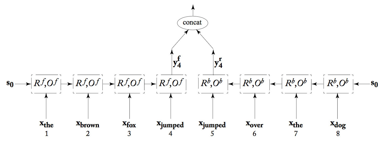
We can join two RNN's together into a "bidirectional RNN." One RNN works forwards from the start of the input, the second works backwards from the end of the input. The output at each position is the concatenation of the two RNN outputs. This combined output would typically receive further processing (not shown) and then eventually be evaluated to produce a loss. When the loss information propagaes backwards, both RNNs receive feedback based on their joint answer.
 from Yoav Goldberg
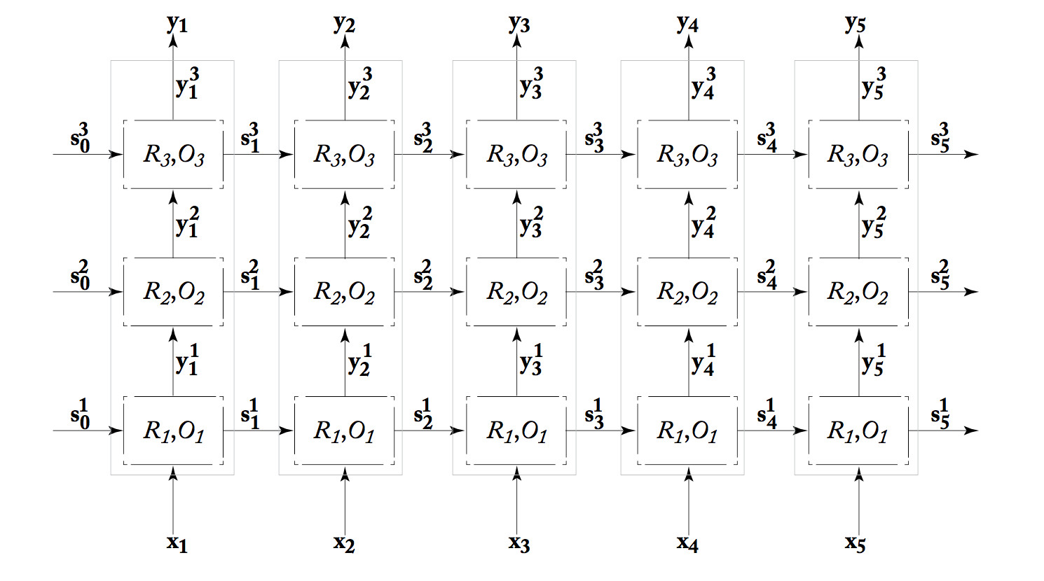
We can also build "deep" RNN's, which have more than one processing layer between the input and output streams. The one shown below has three layers. Because each processing unit in an RNN is already complex (equivalent to multiple units in a standard neural net), it's unusual to see many layers.
 from Yoav Goldberg
In theory, an RNN can remember the entire stream of input values. However, gradient magnitude tends to decay as you move backwards from the loss signal. So earlier inputs may not contributed much to the RNN's final answer at the end. For a transducer, inputs may contribute little to the output for locations some distance away. This is a problem, because many linguistic tasks benefit from an extended context.
To allow RNNs to store information more effectively, researchers use "gated" versions of RNNs. These RNNs include separate vectors (the "gates") which control which parts of the unit's state will be updated at each timestep. The gates make the RNN's behavior easier to control, but create yet more tunable parameters that must be learned. Two popular gated RNN models are the "Long Short-Term Memory" (LSTM) and the "Gated Recurrent Unit" (GRU).
Current training procedures for neural nets still leave them excessively sensitive to small changes in the input data. So it is possible to cook up patterns that are fairly close to random noise but push the network's values towards or away from a particular output classification. Adding these patterns to an input image creates an "adversarial example" that seems almost identical to a human but gets a radically different classification from the network. For example, the following shows the creation of an image that looks like a panda but will be misrecognized as a gibbon.

from Goodfellow et al
The pictures below show patterns of small distortions being used to persuade the network that images from six different types are all ostriches.
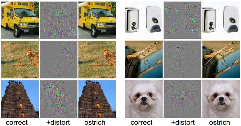
from Szegedy et al.
These pictures come from Andrej Karpathy's blog, which has more detailed discussion.
Clever patterns placed on an object can cause it to disappear, e.g. only the lefthand person is recognized in the picture below.
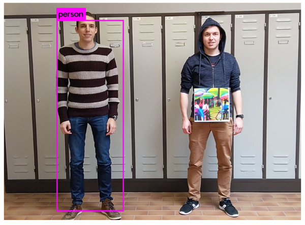
from
Thys, Van Ranst, Goedeme 2019
Disturbingly, the classifier output can be changed by adding a disruptive pattern near the target object. In the example below, a banana is recognized as a toaster.
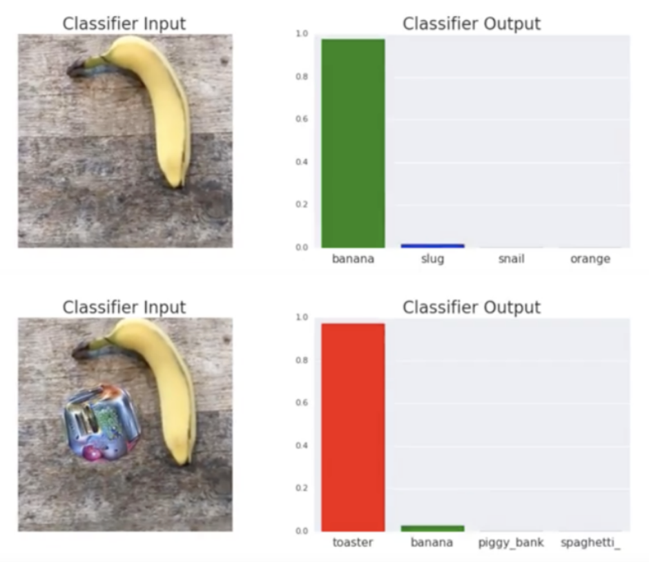
from
Brown, Mane, Roy, Abadi, Gilmer, 2018
And here are a couple more examples of fooling neural net recognizers:
In the words of one researcher (David Forsyth), we need to figure out how to "make this nonsense stop" without sacrificing accuracy or speed. This is currently an active area of research.
Similar adversarial examples can be created purely with text data. In the examples below, the output of a natural language classifier can be changed by replacing words with synonyms. The top example is from a sentiment analysis task, i.e. was this review positive or negative? The bottom example is from a textual entailment task, in which the algorithm is asked to decide how the two sentences are logically related. That is, does one imply the other? Does one contradict the other?
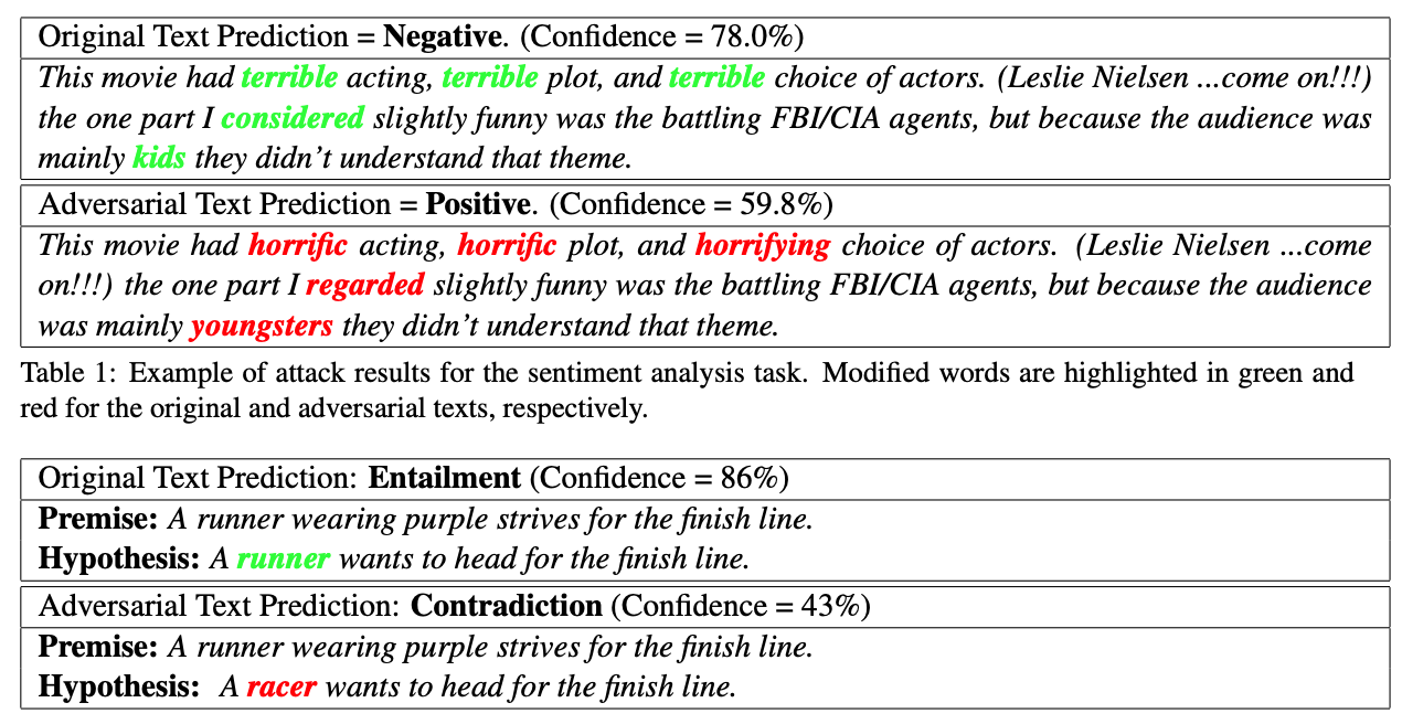
from
Alzantot et al 2018
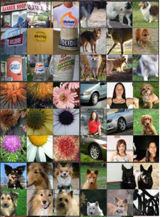
A generative adversarial network (GAN) consists of two neural nets that jointly learn a model of input data. The classifier tries to distinguish real training images from similar fake images. The adversary tries to produce convincing fake images. These networks can produce photorealistic pictures that can be stunningly good (e.g. the dog pictures below) but fail in strange ways (e.g. some of the frogs below).
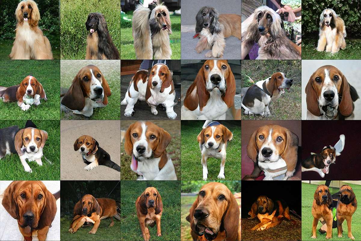
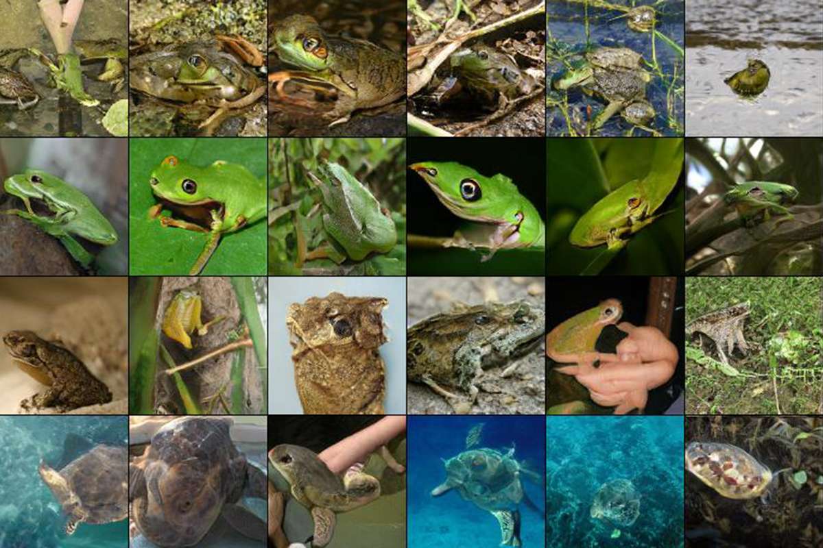
pictures from
New Scientist
article on
Andrew Brock et al research paper
Good outputs are common. However, large enough collections contain some catastrophically bad outputs, such as the frankencat below right. The neural nets seem to be very good at reproducing the texture and local features (e.g. eyes). But they are missing some type of high-level knowledge that tells people that, for example, dogs have four legs.
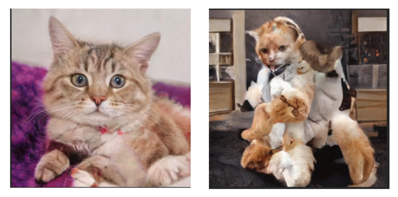
from
medium.com
generated using the tool
https://thiscatdoesnotexist.com/
A recent paper exploited this lack of anatomical understanding to detect GAN-generated faces using the fact that the pupils in the eyes had irregular shapes.
Another fun thing about GANs is that they can learn to hide information in the fine details of images, exploiting the same sensitivity to detail that enables adversarial examples. This GAN was supposedly trained to convert map into arial photographs, by doing a circular task. One half of the GAN translates pictures into arial photographs into maps and the other half translates maps into arial photographs. The output results below are too good to be true:
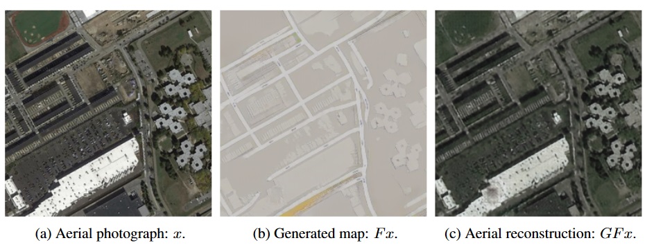
The map-producing half of the GAN is hiding information in the fine details of the maps it produces. The other half of the GAN is using this information to populate the arial photograph with details not present in the training version of the map. Effectively, they have set up their own private communication channel invisible to the researchers (until they got suspicious about the quality of the output images.).
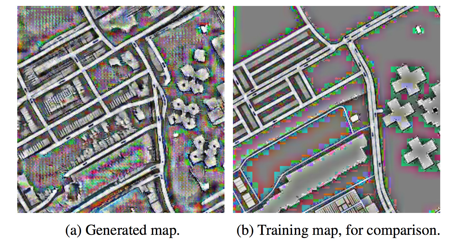
More details are in this Techcrunch summary of Chu, Zhmoginov, Sandler, CycleGAN, NIPS 2017.
Credits to Matt Gormley are from 10-601 CMU 2017
Figures credited to Yoav Goldberg are from his book "Neural Network Methods for Natural Language processing." (If you're on the U. Illinois VPN, you can download it for free.)