Linear classifiers classify input items using a linear combination of feature values. Depending on the details, and the mood and theoretical biases of the author, a linear classifier may be known as
The variable terminology was created by the convergence of two lines of research. One (neural nets, perceptrons) attempts to model neurons in the human brain. The other (logistic regression, SVM) evolved from standard methods for linear regression.
A key limitation of linear units is that class boundaries must be linear. Real class boundaries are frequently not linear. So linear units typically
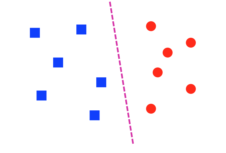
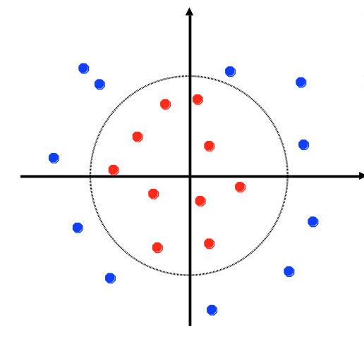
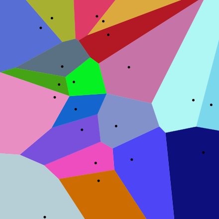
A dataset is linearly separable if we can draw a line (or, in higher dimensions, a hyperplane) that divides one class from the other. The lefthand dataset below is linearly separable; the righthand one is not.
from Lana Lazebnik
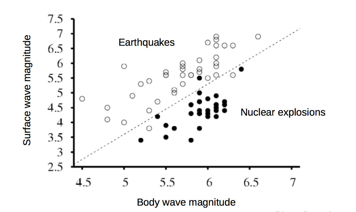
A common situation is that data may be almost linearly separable. That is, we can draw a line that correctly predicts the class for most of the data points, and we can't do any better by adjusting the line. That's often the best that can be done when the data is messy.
from Lana Lazebnik
A single linear unit will try to separate the data with a line/hyperplane, whether or not the data really looks like that.
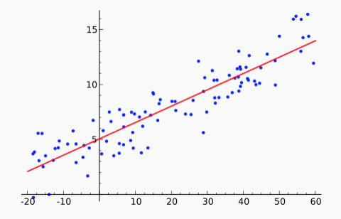
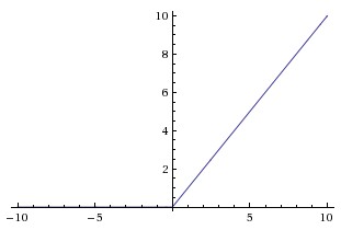
You've probably seen linear regression or, at least, used a canned function that performs it. However, you may well not remember what the term refers to. Linear regression is the process of fitting a linear function f to a set of (x,y) points. That is, we are given a set of data values \(x_i,y_i\). We stipulate that our model f must have the form \(f(x) = ax + b\). We'd like to find values for a and b that minimize the distance between the \(f(x_i)\) and \(y_i\), averaged over all the datapoints. For example, the red line in this figure shows the line f that approximates the set of blue datapoints.
From Wikipedia
There are two common ways to "measure the distance between \(f(x_i)\) and \(y_i\)":
The popular "least squares" method uses the L2 norm. Because this error function is a simple differentiable function of the input, there is a well-known analytic solution for finding the minimum. (See the textbook or many other places.) There are also so-called "robust" methods that minimize the L1 norm. These are a bit more complex but less sensitive to outliers (aka bad input values).
In most classification tasks, our input values are a vector \(\vec{x}\). Suppose that \(\vec{x}\) is two-dimensional, so we're fitting a model function \(f(x_1,x_2)\). A linear function of two input variables must look as follows, where color shows values of the output value \(f(x_1,x_2)\). (red high to blue low).
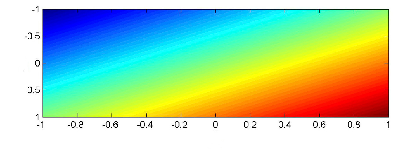 from Mark Hasegawa-Johnson, CS 440, Spring 2018
In classification, we will typically be comparing the output value \(f(x_1,x_2)\). against a threshold T. In this picture, \(f(x_1, x_2) =T\) is a color contour. E.g. perhaps it's the middle of the yellow stripe. The division boundary (i.e. \(f(x_1,x_2) = T\)) is always linear: a straight line for a 2D input, a plane for inputs of higher dimension.
The basic set-up for a linear classifier is shown below. Look at only one class (e.g. pink for cat). Each input example generates a feature vector (x). The four pixel values \(x_1, x_2, x_3, x_4 \) are multiplied by the weights for that class (e.g. the pink cells) to produce a score for that class. A bias term (b) is added to produce the weighted sum \(w_1 x_1 + .... w_n x_n + b \).
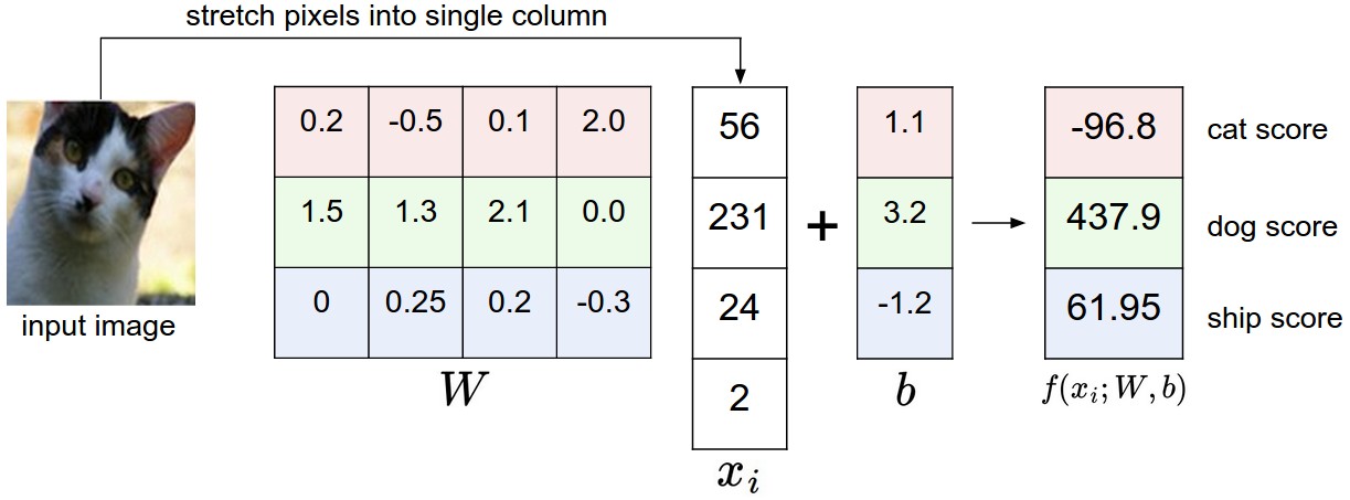
(from Andrej Karpathy cs231n course notes via Lana Lazebnik)
In this toy example, the input features are are individual pixel values. In a real working system, they would probably be something more sophisticated, such as SIFT features or the output of an early stage of neural processing. In a text classifcation task, one might use word or bigram probabilities.
To make a multi-way decision (as in this example), we compare the output values for several classes and pick the class with the highest value. In this toy example, the algorithm makes the wrong choice (dog). Clearly the weights \(w_i\) are key to success.
To make a yes/no decision, we compare the weighted sum to a threshold. The bias term adjusts the output so that we can use a standard threshold: 0 for neural nets and 0.5 for logistic regression. (We'll assume we want 0 in what follows.) In situations where the bias term is notationally inconvenient, we can make it disappear (superficially) by introducing a new input feature \(x_0\) which is tied to the constant 1. Its weight \(w_0\) is the bias term.
In Naive Bayes, we fed a feature vector into a somewhat similar equation (esp. if you think about everything in log space). What's different here?
First, the feature values in Naive Payes were probabilities. E.g. a single number might be the probability of seeing the word "elephant" in some type of text. The values here are just numbers, not in the range [0,1]. We don't know whether all of them are on the same scale.
In naive Bayes, we assumed that features were conditionally independent, given the class label. This may be a reasonable approximation for some sets of features, but it's frequently wrong enough to cause problems. For example, in a bag of words model, "San" and "Francisco" do not occur independently even if you know that the type of text is "restaurant reviews." Logistic regression (a natural upgrade for naive Bayes) allows us to handle features that may be correlated. For example, the individual weights for "San" and "Francisco" can be adjusted so that the pair's overall contribution is more like that of a single word.
Recall that a linear classifier makes its decisions based on a linear combination of the input feature values. That is, if our input features values are \(x_1, x_2, \ldots, x_n\), it tests whether
\(w_1 x_1 + .... w_n x_n + b \ge 0\)
To avoid having to deal separately with the bias term b, we replace this with a fake feature \(x_0\) that is always set to 1, plus an additional weight \(w_0\). So then our decision equation becomes
\(w_0 x_0 + w_1 x_1 + .... w_n x_n \ge 0\)
Reformulating a bit further, let's pass this weighted sum through the sign function (sgn). We'll follow the neural net terminology and call this final function the "activation function." So then our classification is based on this test:
Is \(\text{sgn}(w_0 x_0 + w_1 x_1 + .... w_n x_n ) \) equal to 1 or -1?
We can make one of these units look like a neuron or a circuit component by drawing it like this:
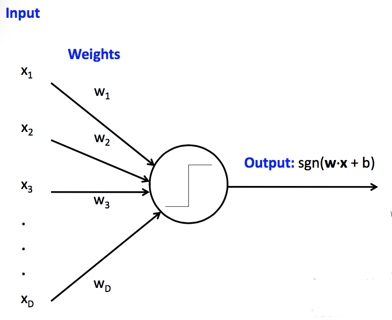 (from Mark Hasegawa-Johnson, CS 440, Spring 2018)
This particular type of linear unit unit is called a perceptron. Perceptrons have limited capabilities but are particularly easy to train.
So far, we've assumed that the weights \(w_0,w_1,\ldots, w_n \) were given to us by magic. In practice, they are learned from training data. Suppose that we have a set T of training data pairs (x,y), where x is a feature vector and y is the (correct) class label. Our training algorithm looks like:
- Initialize weights \(w_0,\ldots, w_n\) to zero
- For some number of iterations through the dataset
- For each training example (x,y), update the weights to improve the changes of classifying x correctly.
Let's suppose that our unit is a classical perceptron, i.e. our activation function is the sign function. Then we can update the weights using the "perceptron learning rule". Suppose that x is a feature vector, y is the correct class label, and \(\hat{y}\) is the class label that was computed using our current weights. Then our update rule is:
- If \(\hat{y}\) = y, do nothing.
- Otherwise \(w_i = w_i + \alpha \cdot y \cdot x_i \)
The "learning rate" constant \(\alpha \) controls how quickly the update process changes in response to new data.
There's several variants of this equation, e.g.
\(w_i = w_i + \alpha \cdot (y-\hat{y}) \cdot x_i \)
When trying to understand why they are equivalent, notice that the only possible values for y and \(\hat{y}\) are 1 and -1. So if \( y = \hat{y} \), then \( (y-\hat{y}) \) is zero and our update rule does nothing. Otherwise, \( (y-\hat{y}) \) is equal to either 2 or -2, with the sign matching that of the correct answer (y). The factor of 2 is irrelevant, because we can tune \( \alpha \) to whatever we wish.
This training procedure will converge if
Apparently convergence is guaranteed if the learning rate is proportional to \(\frac{1}{t}\) where t is the current iteration number. The book recommends a gentler formula: make \(\alpha \) proportional to \(\frac{1000}{1000+t}\).
One run through training data through the update rule is called an "epoch." Training a linear classifier generally uses multiple epochs, i.e. the algorithm sees each training pair several times.
Datasets often have strong local correlations, because they have been formed by concatenating sets of data (e.g. documents) that each have a strong topic focus. So it's often best to process the individual training examples in a random order.
Perceptrons can be very useful but have significant limitations.
Fixes:
- use multiple units (neural net)
- massage input features to make the boundary linear
Fixes:
- reduce learning rate as learning progresses
- don't update weights any more than needed to fix mistake in current example
- cap the maximum change in weights (e.g. this example may have been a mistake)
Fix: switch to a closely-related learning method called a "support vector machines" (SVM's). The big idea for an SVM is that only examples near the boundary matter. So we try to maximize the distance between the closest sample point and the boundary (the "margin").
Perceptrons can easily be generalized to produce one of a set of class labels, rather than a yes/no answer. We use several parallel classifier units. Each has its own set of weights. Join the individual outputs into one output using argmax (i.e. pick the class that has the largest output value).
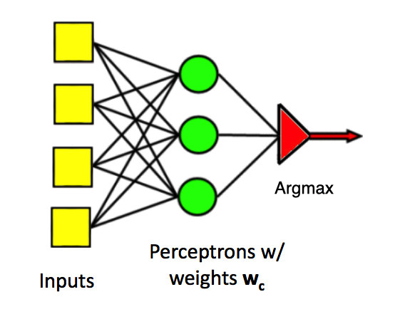
(from Mark Hasegawa-Johnson, CS 440, Spring 2018)
Update rule: Suppose we see (x,y) as a training example, but our current output class is \(\hat{y}\). Update rule:
The classification regions for a multi-class perceptron look like the picture below. That is, each pair of classes is separated by a linear boundary. But the region for each class is defined by several linear boundaries.
from Wikipedia
(from Mark Hasegawa-Johnson, CS 440, Spring 2018)
Classical perceptrons have a step function activation function, so they return only 1 or -1. Our accuracy is the count of how many times we got the answer right. When we generalize to multi-layer networks, it will be much more convenient to have a differentiable output function, so that we can use gradient descent to update the weights.
To do this, we need to separate two functions at the output end of the unit:
For the perceptron, the activation function is the sign function function: 1 if above the threshold, -1 if below it. The loss function for a perceptron is "zero-one loss". We get 1 for each wrong answer, 0 for each correct one.
So our whole classification function is the composition of three functions:
In a multi-layer network, there will be activation functions at each layer and one loss function at the very end.
When we move to differentiable units for making neural nets, the popular choices for differentiable activation functions include the logistic (aka sigmoid), tanh, rectified linear unit (ReLu). Wikipedia has an excessively comprehensive list of alternatives.
The tanh function \( \frac{e^x - e^{-x}}{e^x + e^{-x}} \) looks like this:
 from Mark Hasegawa-Johnson
The logistic/sigmoid function has equation \( \frac{1}{(1+e^{-x})} \). It is just like tanh, except rescaled so that it returns values between 0 and 1 (rather than between -1 and 1). The logistic form would be used when the designer wants to think of the values as probabilities (e.g. logistic regression). Otherwise one would choose whichever is more convenient for later stages of processing.
A rectified linear unit (ReLU) uses the function f, where f(x) = x when positive, f(x) = 0 if negative. It looks like this:
 from
Andrej Karpathy
from
Andrej Karpathy
The activation does not affect the decision from our single, pre-trained unit. Rather, the choice has two less obvious consequences:
Suppose that we have a training pair (x,y). So y is the correct output. Suppose that \(\hat{y}\) is the output of our unit (weighted average and then activation function). Popular differentiable loss functions include
In both cases, our goal is to minimize this loss averaged over all our training pairs.
When using the L2 norm to measure distances (e.g. in a 2D map), one would normally
However, we're just trying to minimize the distance, not actually compute the distance. So we can skip the last (square root) step, because square root is monotonically increasing.
Recall that entropy is the number of bits required to (optimally) compress a pool of values. The high-level idea of cross-entropy is that we have built a model of probabilities (e.g. using some training data) and then use that model to compress a different set of data. Cross-entropy measures how well our model succeeds on this new data. This is one way to measure the difference between the model and the new data.
If you are curious, here is a longer list of loss functions.
Remember the chain rule from calculus. If \(h(x) = f(g(x)) \), the chain rule says that \(h'(x) = f'(g(x))\cdot g'(x) \). In other words, to compute \(h'(x) \), we'll need the derivatives of the two individual functions, plus the value of of them applied to the input.
Let's assume we use the logistic/sigmoid for our activation function and the L2 norm for our loss function.
To work out the update rule for learning weight values, suppose we have a training example (x,y), where x is a vector of feature values. The output with our current weights is
\(\hat{y} = \sigma(w\cdot x)\) where \(\sigma\) is the sigmoid function.
Using the L2 norm as our loss function, our loss from just this one training sample is
\(L(w,x) = (y - \hat{y})^2\)
For gradient descent, we adjust our weights in the opposite of the gradient direction. That is, our update rule for one weight \(w_i\) should look like this, where \(\alpha\) is the learning rate.
\( w_i = w_i - \alpha \cdot \frac{ \partial L(w,x)}{\partial w_i} \)
Let's figure out what \( \frac{ \partial L(w,x)}{\partial w_i} \) is. This requires some patience but is entirely mechanical. It's a calculation that you'll typically ask a software package (e.g. neural net utilities) to do for you.
\( \frac{ \partial L(w,x)}{\partial w_i} = \frac{ \partial (y - \hat{y})^2}{\partial w_i}\) (definition of L(w,x))
= \( 2(y-\hat{y}) \cdot \frac{\partial (y-\hat{y})}{\partial{w_i}} \) (chain rule)
= \( 2(y-\hat{y}) \cdot \frac{\partial (- \hat{y})}{\partial{w_i}} \) (y doesn't depend on \(w_i\)) = \( -2(y-\hat{y}) \cdot \frac{\partial \hat{y}}{\partial{w_i}} \) (y doesn't depend on \(w_i\))
OK, so now what is \(\frac{\partial \hat{y}}{\partial{w_i}} \)? If we look up the derivative of the sigmoid function, we find that \(\frac{\partial \sigma(z)}{\partial z} = \sigma(z)(1-\sigma(z))\). Using this fact:
\(\frac{\partial \hat{y}}{\partial{w_i}} \) = \(\frac{\partial \sigma(w\cdot x)}{\partial{w_i}} \) (definition of \(\hat{y}\))
= \(\sigma(w\cdot x)\cdot(1-\sigma(w\cdot x))\cdot\frac{\partial w\cdot x}{\partial w_i}\) (chain rule and the derivative of \(\sigma\))
= \(\sigma(w\cdot x)\cdot (1-\sigma(w\cdot x))\cdot x_i\) (it's just a polynomial)
= \(\hat{y}\cdot (1-\hat{y})\cdot x_i\) (definition of \(\hat{y}\))
Substituting this into our earlier formula, we get
\( \frac{ \partial L(w,x)}{\partial w_i} = -2\cdot (y-\hat{y})\cdot \hat{y}\cdot (1-\hat{y})\cdot x_i\)
So our update formula is
\( w_i = w_i + 2\alpha \cdot (y-\hat{y})\cdot \hat{y}\cdot (1-\hat{y})\cdot x_i\)
\(\alpha\) is just a tuning parameter, so we can fold 2 into it. This gives us our final update equation:
\( w_i = w_i + \alpha \cdot (y-\hat{y})\cdot \hat{y}\cdot (1-\hat{y})\cdot x_i\)
Ugly, unintuitive, but straightforward to code.
Recall how we built a multi-class perceptron. We fed each input feature to all of the units. Then we joined their outputs together with an argmax to select the class with the highest output.
(from Mark Hasegawa-Johnson, CS 440, Spring 2018)
We'd like to do something similar with differentiable units.
There is no (reasonable) way to produce a single output variable that takes discrete values (one per class). So we use a "one-hot" representation of the correct output. A one-hot representation is a vector with one element per class. The target class gets the value 1 and other classes get zero. E.g. if we have 8 classes and we want to specify the third one, our vector will look like:
[0, 0, 1, 0, 0, 0, 0, 0]
One-hot doesn't scale well to large sets of classes, but works well for medium-sized collections.
Now, suppose we have a sequence of classifier outputs, one per class. \(v_1,\ldots,v_n\). We often have little control over the range of numbers in the \(v_i\) values. Some might even be negative. We'd like to map these outputs to a one-hot vector. Softmax is a differentiable function that approximates this discrete behavior. It's best thought of as a version of argmax.
Specifically, softmax maps each \(v_i\) to \(\displaystyle \frac{e^{v_i}}{\sum_i e^{v_i}}\). The exponentiation accentuates the contrast between the largest value and the others, and forces all the values to be positive. The denominator normalizes all the values into the range [0,1], so they look like probabilities (for folks who want to see them as probabilities).