
a real-world trellis (supporting a passionfruit vine)
Hidden Markov Models are used in a wide range of applications. They are similar to Bayes Nets (both being types of "Graphical Models"). We'll see them in the context Part of Speech tagging. Uses in other applications (e.g. speech) look very similar.
We saw part-of-speech (POS) tagging in a previous lecture. Recall that we start with a sequence of words. The tagging algorithm needs to decorate each word with a part-of-speech tag. Here's an example:
INPUT: Northern liberals are the chief supporters of civil rights and of integration. They have also led the nation in the direction of a welfare state.
OUTPUT: Northern/jj liberals/nns are/ber the/at chief/jjs supporters/nns of/in civil/jj rights/nns and/cc of/in integration/nn ./. They/ppss have/hv also/rb led/vbn the/at nation/nn in/in the/at direction/nn of/in a/at welfare/nn state/nn ./.
Identifying a word's part of speech provides strong constraints on how later processing should treat the word. Or, viewed another way, the POS tags group together words that should be treated similarly in later processing. For example, in building parse trees, the POS tags povide direct information about the local syntactic structure, reducing the options that the parse must choose from.
Many early algorithms exploit POS tags directly (without building a parse tree) because the POS tag can help resolve ambiguities. For example, when translating, the noun "set" (i.e. collection) would be translated very differently from the verb "set" (i.e. put). The part of speech can distinguish words that are written the same but pronounced differently, such as:
POS tag sets vary in size, e.g. 87 in the Brown corpus down to 12 in the "universal" tag set from Petrov et all 2012 (Google research). Even when the number of tags is similar, different designers may choose to call out different linguistic distinctions.
| our MP | "Universal" | Our MP |
|---|---|---|
| NOUN | Noun | noun |
| PRON | Pronoun | pronoun |
| VERB | Verb | verb |
| MODAL | modal verb | |
| ADJ | Adj | adjective |
| DET | Det | determiner or article |
| PERIOD | . (just a period) | end of sentence punctuation |
| PUNCT | other punctuation | |
| NUM | Num | number |
| IN | Adp | preposition or postposition |
| PART | particle e.g. after verb, looks like a preposition) | |
| TO | infinitive marker | |
| ADV | Adv | adverb |
| Prt | sentence particle (e.g. "not") | |
| UH | [not clear what tag] | filler, exclamation |
| CONJ | Conj | conjunction |
| X | X | other |
Here's a more complex set of 36 tags from the
Penn Treebank tagset .
The larger tag sets are a mixed blessing. On the one hand, the
tagger must make finer distinctions when it chooses the tag.
On the other hand, a more specific tag provides more information
for tagging later words and also for subsequent processing (e.g. parsing).
Each word has several possible tags, with different probabilities.
For example, "can" appears using in several roles:
Some other words with multiple uses
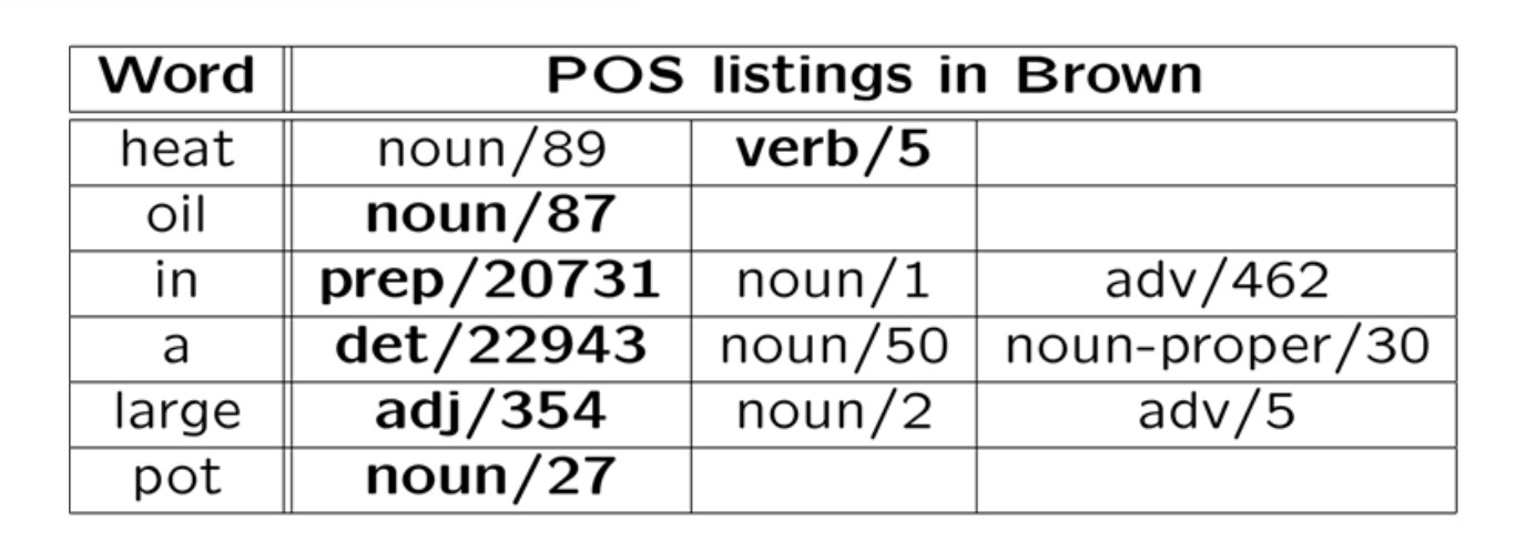
Consider the sentence "Heat oil in a large pot." The correct tag sequence
is "verb noun prep det adj noun". Here's the tags seen when training
on the Brown corpus.
Notice that
An example of that last would be "over" used as a noun (e.g. in cricket).
That is fairly common in British text but might never occur in a training corpus
from the US.
Most testing starts with a "baseline" algorithm, i.e. a simple
method that does do the job, but typically not very well. In this
case, our baseline algorithm might pick the most common tag for
each word, ignoring context. In the table above, the most common
tag for each word is shown in bold: it made one error out of six
words.
The test/development data will typically contain some words that weren't
seen in the training data. The baseline algorithm guesses that these
are nouns, since that's the most common tag for infrequent words. An
algorithm can figure this out by examining new words that appear in the
development set, or by examining the set of words that occur only once
in the training data ("hapax") words.
On larger tests, this baseline algorithm has an accuracy around 91%.
It's essential for a proposed new algorithm to beat the baseline. In
this case, that's not so easy because the baseline performance is
unusually high.
Suppose that W is our input word sequence (e.g. a sentence) and T is
an input tag sequence. That is
Our goal is to find a tag sequence T that maximizes P(T | W).
Using Bayes rule, this is equivalent to maximizing \( P(W \mid T) * P(T)/P(W) \)
And this is equivalent to maximizing \( P(W \mid T) * P(T) \) because P(W) doesn't depend
on T.
So we need to estimate P(W | T) and P(T) for one fixed word
sequence W but for all choices for the tag sequenceT.
Obviously we can't directly measure the probability of an entire sentence
given a similarly long tag sequence. Using (say) the Brown corpus,
we can get reasonable estimates for
If we have enough tagged data, we can also estimate tag trigrams.
Tagged data is hard to get in quantity, because human intervention is needed
for checking and correction.
To simplify the problem, we make "Markov assumptions." A Markov
assumption is that the value of interest depends only on a short
window of context. For example, we might assume that the probability
of the next word depends only on the two previous words. You'll often
see "Markov assumption" defined to allow only a single item of
context. However, short finite contexts can easily be simulated using
one-item contexts.
For POS tagging, we make two Markov assumptions. For each position
k:
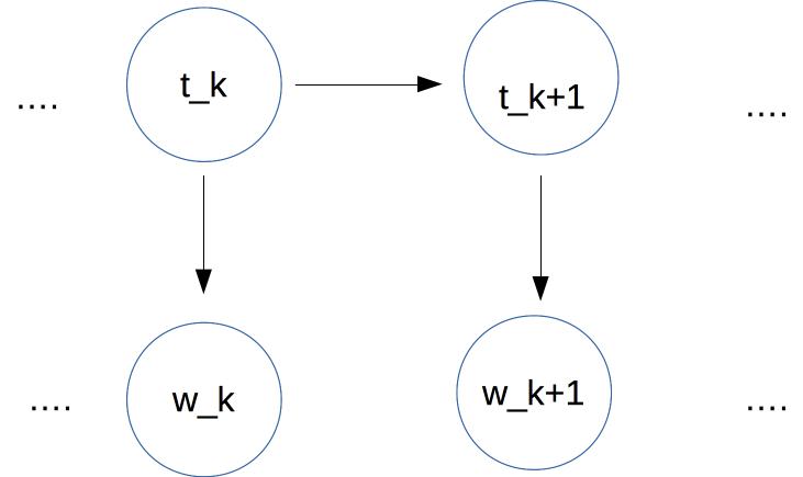
Like Bayes nets, HMMs are a type of graphical model and so we can use
similar pictures to visualize the statistical dependencies:
In this case, we have a sequence of tags at the top. Each
tag depends only on the previous tag. Each
word (bottom row) depends only on the corresonding tag.
Therefore
where \( P(t_1 | START) \) is the probability of tag \(t_1\) at the start of
a sentence.
Folding this all together,
we're finding the T that maximizes
Let's label our probabilities as \(P_S\), \(P_E\), and \(P_T\) to make
their roles more explicit. Using this notation, we're trying to maximize
So we need to estimate three types of parameters:
For simplicity, let's assume that we have only three tags:
Noun, Verb, and Determiner (Det). Our input will contain
sentences that use only those types of words, e.g.
We can look up our initial probabilities, i.e. the probability
of various values for \(P_S(t_1)\)
in a table like this.
We can estimate these by counting how often each tag occurs
at the start of a sentence in our training data.
In the (correct) tag sequence for this sentence,
the tags \(t_1\) and \(t_5\) have the same
value Det. So
the possibilities for the following tags (\(t_2\) and \(t_6\))
should be similar.
In POS tagging, we assume that \(P_T(t_{k+1} \mid t_k)\)
depends only on the identities of \(t_{k+1}\) and \( t_k\), not on
their time position k. (This is a common assumption for Markov
models.)
This is not an entirely safe assumption. Noun phrases early in a
sentence are systematically different from those toward the end.
The early ones are more likely to be pronouns or short noun phrases
(e.g. "the bike"). The later ones more likely to contain nouns that
are new to the conversation and, thus, tend to be more elaborate
(e.g. "John's fancy new racing bike"). However, abstracting away
from time position is a very useful simplifying assumption which
allows us to estimate parameters with realistic amounts of training
data.
So, suppose we need to find a transition probability
\( P_T(t_k | t_{k-1}) \) for two tags
\(t_{k-1} \) and \(t_k \) in our tag sequence.
We consider only the identities of the two tags,
e.g. \(t_{k-1} \) might be DET and
\(t_k \) might be NOUN. And we look up the pair of tags
in a table like this
We can estimate these by counting how often a 2-tag sequence (e.g. Det Noun)
occurs and dividing by how often the first tag (e.g. Det) occurs.
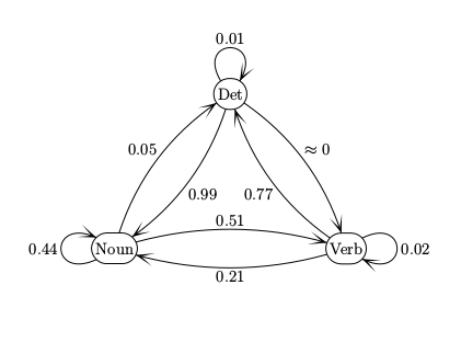
Notice the near-zero probability of a transition from Det to Verb.
If this is actually zero in our training data, do we want to use
smoothing to fill in a non-zero number? Yes, because
even "impossible" transitions may occur in real data due to
typos or (with larger tagsets) very rare tags. Laplace smoothing should work well.
We can view the transitions between tags as a finite-state automaton (FSA).
The numbers on each arc is the probability of that transition happening.
These are conceptually the same as the FSA's found in CS theory courses.
But beware of small differences in conventions.
Our final set of parameters are the emission probabilities, i.e. \(P_E(w_k | t_k)\)
for each position k in our tag sequence.
Suppose we have a very small vocabulary of nouns and verbs to go with our toy
model. Then we might have probabilities like
Because real vocabularies are very large, it's common to see new
words in test data. So it's essential to smooth, i.e. reserve some
of each tag's probability for
New tags for a familiar word are quite common in English, because most nouns
can be used as verbs, and vice versa.
However, the details may need to depend on the type of tag. Tags
divide (approximately) into two types
It's very common to see new open-class words. In English,
open-class tags for existing words are also likely, because nouns
are often repurposed as verbs, and vice versa. E.g. the proper name
MacGyver
spawned a verb, based on the improvisational skills of the
TV character with that name. So open class tags need to reserve
significant probability mass for unseen words, e.g. larger Laplace
smoothing constant.
It's possible to encounter new closed-class words, e.g. "abaft."
But this is much less common than new open-class words.
So these tags should have a smaller Laplace smoothing constant.
The amount of probability mass to reserve for each tag
can be estimated by looking at the
tags of "hapax" words (words that occur only once) in our training data.
Once we have estimated the model parameters, the Viterbi algorithm
finds the highest-probability tag sequence for each input word
sequence. Suppose that our input word sequence is \(w_1,\ldots w_n\).
The basic data structure is an n by m array (v), where n is the
length of the input word sequence
and m is the number of different (unique) tags. Each cell
(k,t) in the array contains the probability
v(k,t) of the best sequence of
tags for \(w_{1}\ldots w_{k} \)
that ends with tag t.
We also store b(k,t), which is the previous tag in that best sequence.
This data structure is called a "trellis."
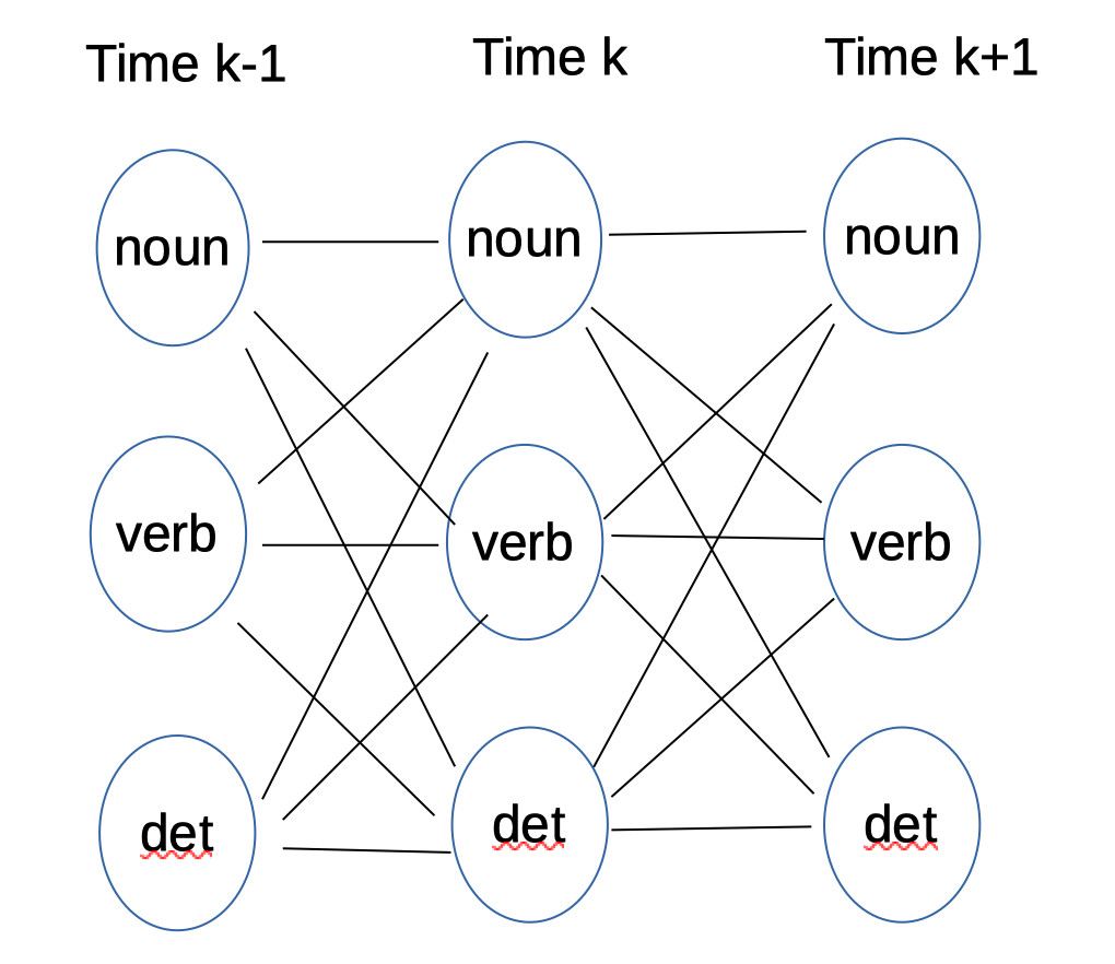
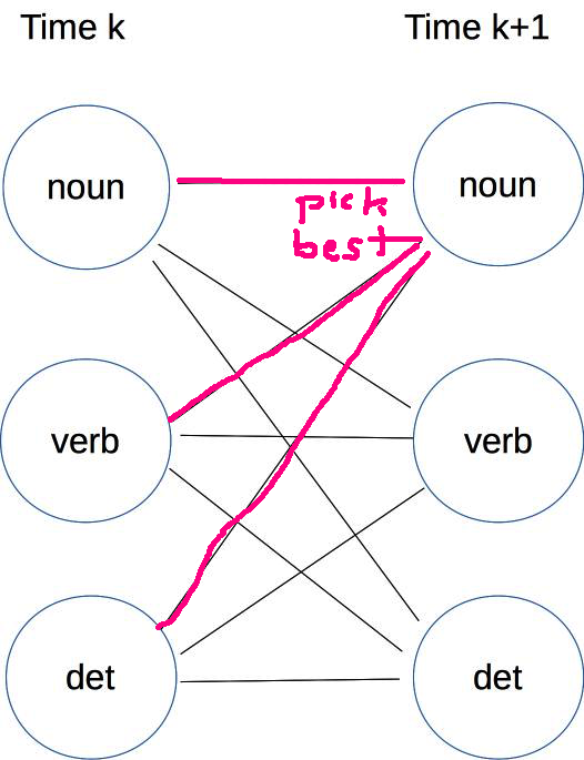
Here's a picture of one section of the trellis, drawn as a graph.
It's called a trellis because it resembles trellises used to support
plants in the real world. (This one is supporting a passionfruit vine.)
Tags and words
 (from Mitch Marcus)
Baseline algorithm
Formulating the estimation problem
\(W = w_1, w_2, \ldots w_n \)
\(T = t_1, t_2, \ldots t_n \)
What can we realistically estimate?
Markov assumptions
\(P(w_k)\) depends only on \(P(t_k)\)
\(P(t_k) \) depends only on \(P(t_{k-1}) \)
The equations
\( P(W \mid T) = \prod_{i=1}^n P(w_i \mid t_i)\)
\( P(T) = P(t_1 | START) * \prod_{i=1}^n P(t_k \mid t_{k-1}) \)
\( P (T \mid W)\)
\(\propto P(W \mid T) * P(T) \)
\( = \prod_{i=1}^n P(w_i \mid t_i)\ \ * \ \
P(t_1 \mid \text{START})\ \ *\ \ \prod_{k=2}^n P(t_k \mid t_{k-1}) \)
\( \prod_{i=1}^n P_E(w_i \mid t_i)\ \ * \ \
P_S(t_1)\ \ *\ \ \prod_{k=2}^n P_T(t_k \mid t_{k-1}) \)
Toy model
    Det Noun     Verb    Det Noun   Noun
    The student  ate     the ramen  noodles
    Det Noun   Noun  Verb    Det Noun
    The maniac rider crashed his bike.
tag
\(P_S(tag)\)
Verb
0.01
Noun
0.18
Det
0.81
Transition probabilities
Next Tag
Previous tag
Verb
Noun
Det
Verb
0.02
0.21
0.77
Noun
0.51
0.44
0.05
Det
\(\approx 0 \)
0.99
0.01
Finite-state automaton
Emission probabilities
   Verb   played 0.01
          ate   0.05
          wrote 0.05
          saw   0.03
          said  0.03
          tree  0.001

   Noun  boy   0.01
         girl  0.01
         cat   0.02
         ball  0.01
         tree  0.01
         saw   0.01

   Det  a    0.4
        the  0.4
        some 0.02
        many 0.02
The trellis
|
|
A path ending in some specific tag at time k might continue to any one of the possible tags at time k+1. So each cell in column k is connected to all cells in column k+1. The name "trellis" comes from this dense pattern of connections between each timestep and the next.
The Viterbi algorithm fills the trellis from left to right, as follows:
Initialization: We fill the first column using the initial probabilities. Specifically, the cell for tag t gets the value \( v(1,t) = P_S (t) * P_E(w_1 \mid t) \).
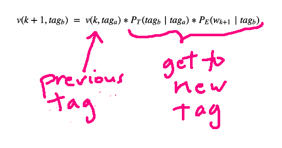
Moving forwards in time: Use the values in column k to fill column k+1. Specifically
For each tag \(tag_B\)That is, we compute \(v(k, tag_A) * P_T(tag_B \mid tag_A) * P_E(w_{k+1} \mid tag_B) \) for all possible tags \(tag_A\). The maximum value goes into trellis cell \( v(k+1,tag_B) \) and the corresponding value of \(tag_A\) is stored in \( b(k+1,tag_B) \).\( v(k+1,tag_B) = \max_{tag_A}\ \ v(k, tag_A) * P_T(tag_B \mid tag_A) * P_E(w_{k+1} \mid tag_B) \)
\( b(k+1,tag_B) = \text{argmax}_{tag_A}\ \ v(k, tag_A) * P_T(tag_B \mid tag_A) * P_E(w_{k+1} \mid tag_B) \)Finishing: When we've filled the entire trellis, pick the best tag (highest v value) T in the final (time=n) column. Trace backwards from T, using the values in b, to produce the output tag sequence.
For example, suppose that we're trying to compute the v and b values for the noun tag at time k+1. We look at all of the cells for the previous timestep, considering their v value, the probability of a transition from that tag to the tag noun, and the emission probability for tag noun given the word at time k+1. We pick the previous cell that gives us the best value for v(k+1,noun) and set b to be the corresponding tag at time k.
The Viterbi algorithm depends on this mystery rule for computing a value at time k+1 from a value at time k.
\( v(k+1,tag_b) \ = \ v(k,tag_a) * P_T(tag_b \mid tag_a) * P_E(w_{k+1} \mid tag_b) \)
What is it?
We can think of the Viterbi algorithm as searching the trellis like a maze, but consistently moving from left to right (i.e. following the progression of time). The righthand side of our equation is the product of two terms:
As we move through the trellis, we're multiplying costs, where we would add them in a normal maze. And we're maximizing probability rather than minimizing cost. But the main structure of the method is similar. And we produce the final output path by tracing backwards, just as we would in a maze search algorithm.
Fairly common to add dummy START and END words to the start and end of each sentence. These would have tags START and END. Then \(P_s\) has a very simple form, since the only legal tag is START.
The probabilities in the Viterbi algorithm can get very small, creating a real possibility of underflow. So the actual implementation needs to convert to logs and replace multiplication with addition. After the switch to addition, the Viterbi computation looks even more like edit distance or maze search. That is, each cell contains the cost of the best path from the start to our current timestep. As we move to the next timestep, we're adding some additional cost to the path. However, for Viterbi we prefer larger, not smaller, values.
The asymptotic running time for this algorithm is \( O(m^2 n) \) where n is the number of input words and m is the number of different tags. In typical use, n would be very large (the length of our test set) and m fairly small (e.g. 36 tags in the Penn treebank). Moreover, the computation is quite simple. So Viterbi ends up with good constants and therefore a fast running time in practice.
The Viterbi algorithm can be extended in several ways. First, high accuracy taggers typically use two tags of context to predict each new tag. This increases the height of our trellis from m to \(m^2\). So the full trellis could become large and expensive to computer. These methods typically use beam search, i.e. keep only the most promising trellis states for each timestep.
So far, we've been assuming that all unseen words should be treated as unanalyzable unknown objects. However, the form of a word often contains strong cues to its part of speech. For example, English words ending in "-ly" are typically adverbs. Words ending in "-ing" are either nouns or verbs. We can use these patterns to make more accurate guesses for emission probabilities of unseen words.
Finally, suppose that we have only very limited amounts of tagged training data, so that our estimated model parameters are not very accurate. We can use untagged training data to refine the model parameters, using a technique called the forward-backward (or Baum-Welch) algorithm. This is an application of a general method called "Expectation Maximization" (EM) and it iteratively tunes the HMM's parameters so as to improve the computed likelihood of the training data.
Here is an interesting example from 1980 of how an HMM can automatically learn sound classes: R. L. Cave and L. P. Neuwirth, "Hidden Markov models for English."
Chapter 8 of Jurafsky and Martin
Chapter 14 of Forsyth's Probability and Statistics (Access from inside the UIUC network.)