Game search differs in several ways from the types of search we've seen so far.
For example, chess has about 35 moves from any board configuration. A game may be 100 ply deep. So the full search tree could contain about \(35^{100}\) nodes which is about \(10^{154}\) nodes.
→ What is a "ply"? This is game computing jargon for one turn by one player. A "move" is a sequence of plies in which each player has one turn. This terminology is consistent with common usage for some, but not all, games.
The large space of possibilities makes games difficult for people, so performance is often seen as a measure of intelligence. In the early days, games were seen as a good domain for computers to demonstrate intelligence. However, it has become clear that the precise definitions of games make them comparatively easy to implement on computers. AI has moved more towards practical tasks (e.g. cooking) as measures of how well machines can model humans.
Game performance is heavily dependent on search and, therefore, high-performance hardware. Scrabble programs beat humans even back in the 1980's. More games have become doable. The graph below shows how computer performance on chess has improved gradually, so that the best chess and go programs now beat humans. High-end game systems have become a way for computer companies to show off their ability to construct an impressive array of hardware.
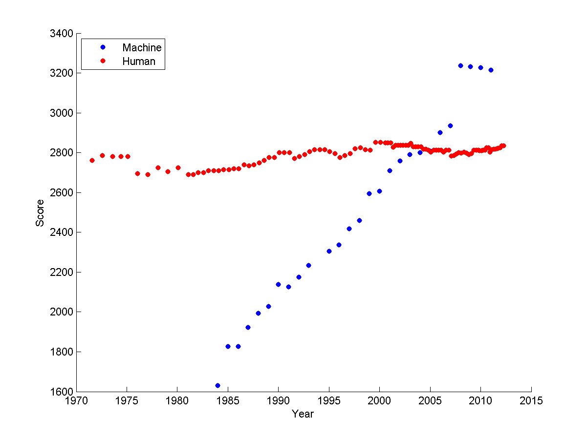
chess Elo ratings over time
from
Sarah Constantin
Games come in a wide range of types. The most basic questions that affect the choice of computer algorithm are:
| fully observable? | determininistic? | size | |
|---|---|---|---|
| Tic-tac-toe | yes | yes | small |
| Chess | yes | yes | big |
| Monopoly | yes | no | big |
| Poker | no | no | big |
Some other important properties:
What is zero sum? Final rewards for the two (or more) players sum to a constant. That is, a gain for one player involves equivalent losses for the other player(s) This would be true for games where there are a fixed number of prizes to accumulate, but not for games such as scrabble where the total score rises with the skill of both players.
Normally we assume that the opponent is going to play optimally, so we're planning for the worst case. Even if the opponent doesn't play optimally, this is the best approach when you have no model of the mistakes they will make. If you do happen to have insight into the limitations of their play, those can be modelled and exploited.
Time limits are most obvious for competitive games. However, even in a friendly game, your opponent will get bored and walk away (or turn off your power!) if you take too long to decide on a move.
Many video games are good examples of dyanmic environments. If the changes are fast, we might need to switch from game search to methods like reinforcement learning, which can deliver a fast (but less accurate) reaction.
We'll normally assume zero sum, two players, static, large (but not infinite) time limit. We'll start with deterministic games and then consider stochastic ones.
Games are typically represented using a tree. Here's an example (from Mitch Marcus at U. Penn) of a very simple game called Hexapawn, invented by Martin Gardner in 1962.
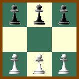
This game uses the two pawn moves from chess (move forwards into an empty square or move diagonally to take an opposing piece). A player wins if (a) he gets a pawn onto the far side, (b) his opponent is out of pawns, or (c) his opponent can't move.
The top of the game tree looks as follows. Notice that each layer of the tree is a ply, so the active player changes between successive levels.
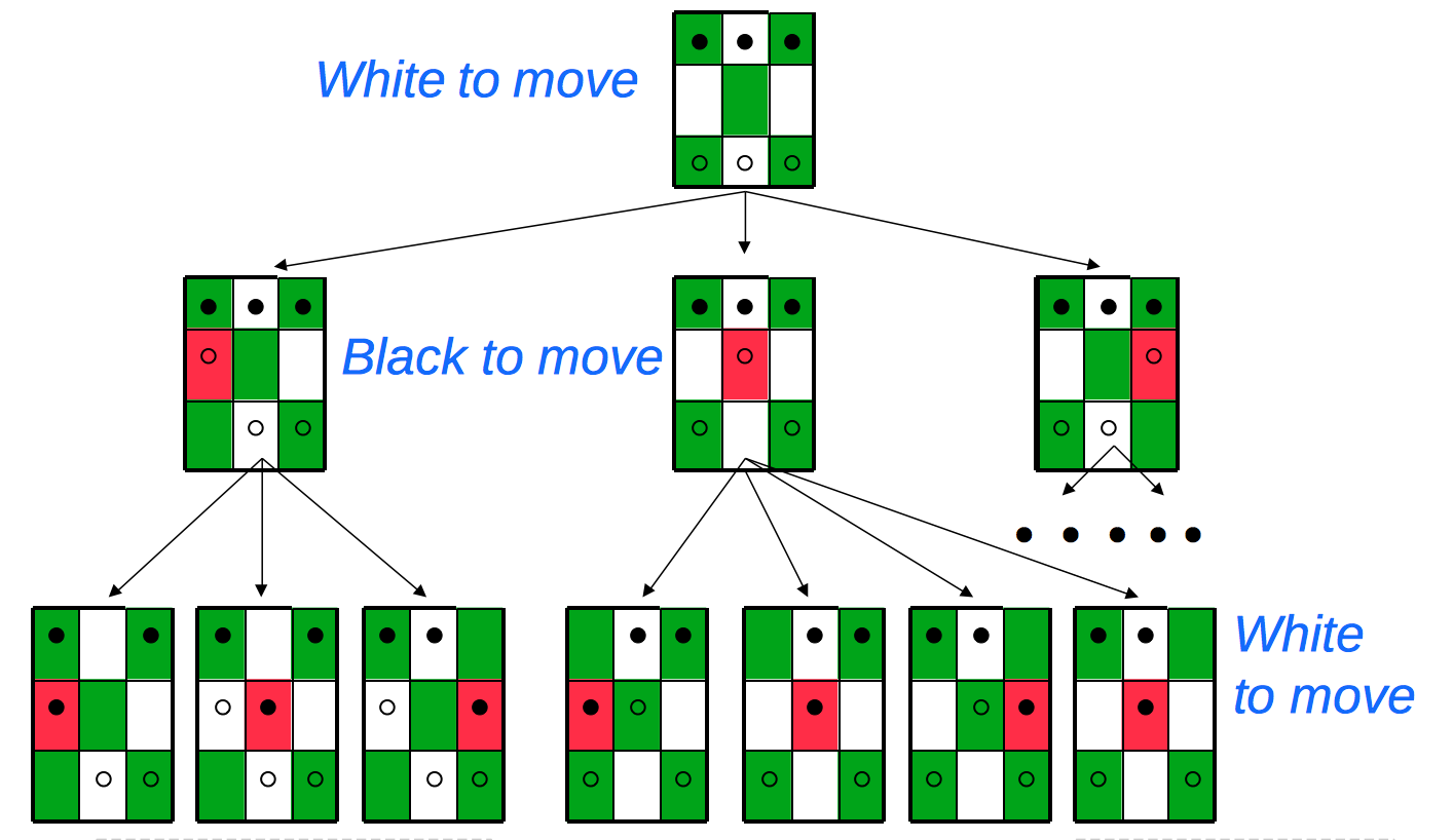
Notice that a game "tree" may contain nodes with identical contents. So we might actually want to treat it as a graph. Or, if we stick to the tree represenation, memoize results to avoid duplicating effort.
Here's the start of the game tree for a more complex game, tic-tac-toe.
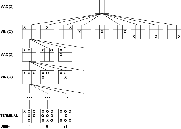
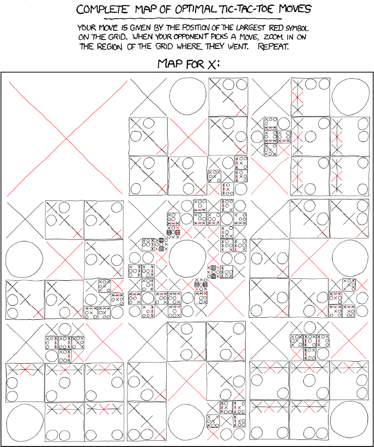
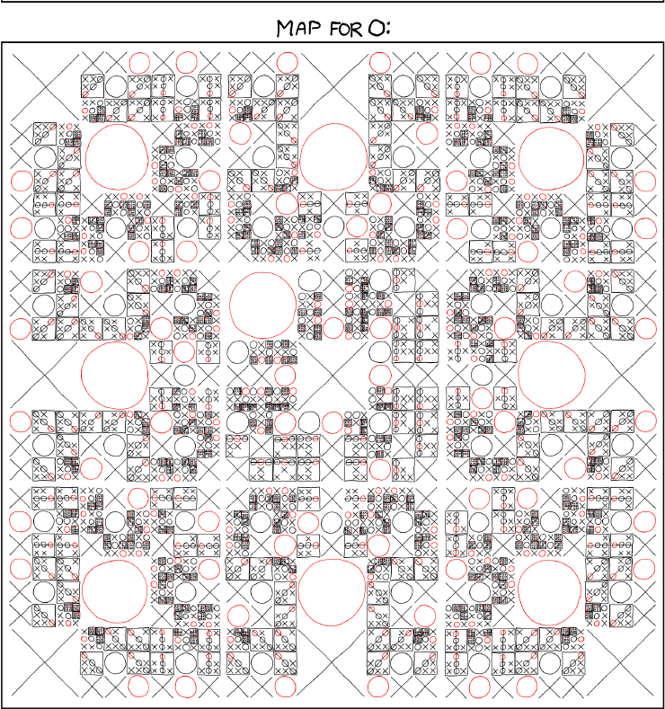
Tic-tac-toe is still simple enough that we can expand out the entire tree of possible moves, finding out that either player can force a draw. It's slightly difficult for humans to do this without making mistakes, but computers are good at this kind of bookkeeping. The first computer implementation was in 1952 on the EDSAC computer. Here's the details, compacted into a convenient diagram by the good folks at xkcd.
Game search uses a combination of two techniques:
Let's consider how to do adversarial search for a two player, deterministic, zero sum game. For the moment, let's suppose the game is simple enough that we can can build the whole game tree down to the bottom (leaf) level. Also suppose we expect our opponent to play optimally (or at least close to).
Traditionally we are called max and our opponent is called min. The following shows a (very shallow) game tree for some unspecified game. The final reward values for max are shown at the bottom (leaf) level.
max                             *
                       /        |    \
                  /             |        \
               /                |             \
min        *                    *                 *
          /  \             /    |    \          /   \
max     *      *          *     *     *        *      *
       /|\     |\        /\    /\    /\        |\    /\
      4 2 7    3 1       5 8   2 9   5 6       1 2   3 5
Minimax search propagates values up the tree, level by level, as follows:
In our example, at the first level from the bottom, it's max's move. So he picks the highest of the available values:
max                             *
                       /        |    \
                  /             |        \
               /                |             \
min        *                    *                 *
          /  \             /    |    \          /   \
max     7      3          8     9     6        2     5
       /|\     |\        /\    /\     /\       |\    /\
      4 2 7    3 1      5  8   2 9   5 6       1 2   3 5
At the next level (moving upwards) it's min's turn. Min gains when we lose, so he picks the smallest available value:
max                             *
                       /        |    \
                  /             |        \
               /                |             \
min        3                    6                 2
          /  \             /    |    \          /   \
max     7      3          8     9     6        2     5
       /|\     |\        /\     /\    /\       |\    /\
      4 2 7    3 1      5  8   2 9   5 6       1 2   3 5
The top level is max's move, so he again picks the largest value. The double hash signs (##) show the sequence of moves that will be chosen, if both players play optimally.
max                             6
                       /       ##    \
                  /            ##        \
               /               ##             \
min        3                /   6 ##              2
          /  \             /    |   ##          /   \
max     7      3          8     9     6        2      5
       /|\     |\        /\    /\    / ##      |\    /\
      4 2 7    3 1      5  8   2 9   5  6      1 2   3 5
This procedure is called "minimax" and is optimal against an optimal opponent. Usually our best choice even against suboptimal opponents unless we have special insight into the ways in which they are likely to play badly.
Minimax search extends to cases where we have more than two players and/or the game is not zero sum. In the fully general case, each node at the bottom contains a tuple of reward values (one per player). At each level/ply, the appropriate player choose the tuple that maximizes their reward. The chosen tuples propagate upwards in the tree, as shown below.
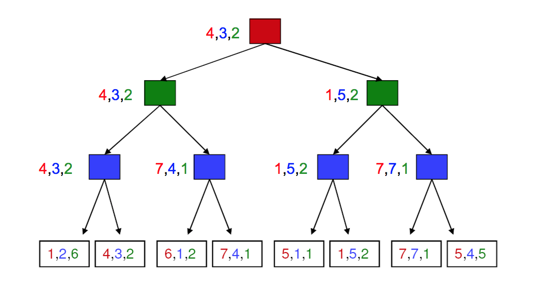
from Lana Lazebnik.
Red plays first, then green, then blue. Score triples are in the same order.
For more complex games, we won't have the time/memory required to search the entire game tree. So we'll need to cut off search at some chosen depth. In this case, we heuristically evaluate the game configurations in the bottom level, trying to guess how good they will prove. We then use minimax to propagate values up to the top of the tree and decide what move we'll make.
As play progresses, we'll know exactly what moves have been taken near the top of the tree. Therefore, we'll be able to expand nodes further and further down the game tree. When we see the final result of the game, we can use that information to refine our evaluations of the intermediate nodes, to improve performance in future games.
Here's a simple way to evaluate positions for tic-tac-toe. At the start of the game, there are 8 ways to place a line of three tokens. As play progresses, some of these are no longer available to one or both players. So we can evaluate the state by
f(state) = [number of lines open to us] - [number of lines open to opponent]
The figure below shows the evaluations for early parts of the game tree:
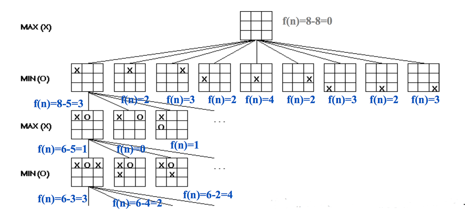
(from Mitch Marcus again)
Evaluations of chess positions dates back to a simple proposal by Alan Turing. In this method, we give a point value to each piece, add up the point values, and consider the difference between our point sum and that of our opponent. Appropriate point values would be
We can do a lot better by considering "positional" features, e.g. whether a piece is being threatened, who has control over the center. A weighted sum of these feature values would be used to evaluate the position. The Deep Blue chess program has over 8000 positional features.
More generally, evaluating a game configuration usually involves a weighted sum of features. In early systems, the features were hand-crafted using expert domain knowledge. The weighting would be learned from databases of played games and/or by playing the algorithm against itself. (Playing against humans is also useful, but can't be done nearly as many times.) In more recent systems, both the features and the weighting may be replaced by a deep neural net.
Something really interesting might happen just after the cutoff depth. This is called the "horizon effect." We can't completely stop this from happening. However, we can heuristically choose to stop search somewhat above/below the target depth rather than applying the cutoff rigidly. Some heuristics include:
Two other optimizations are common:
A table of stored positions is often called a "transposition table" because a common way to hit the same state twice is to have two moves (e.g. involving unrelated parts of the board) that can be done in either order.
from Berkeley CS 188 slides
Each tree node represents a game state. As imagined by a theoretician, we might use the following bottom-up approach to finding our best move:
As we'll see soon, we can often avoid building out the entire game tree (even to depth d). So a better approach to implementation uses recursive depth-first search. So the algorithm for finding our best move actually looks like:
How do we make this process more effective?
Idea: we can often compute the utility of the root without examining all the nodes in the game tree.
Once we've seen some of the lefthand children of a node, this gives us a preliminary value for that node. For a max node, this is a lower bound on the value at the node. For a min node, this gives us an upper bound. Therefore, as we start to look at additional children, we can abandon the exploration once it becomes clear that the new child can't beat the value that we're currently holding.
Here's an example from from Diane Litman (U. Pitt).
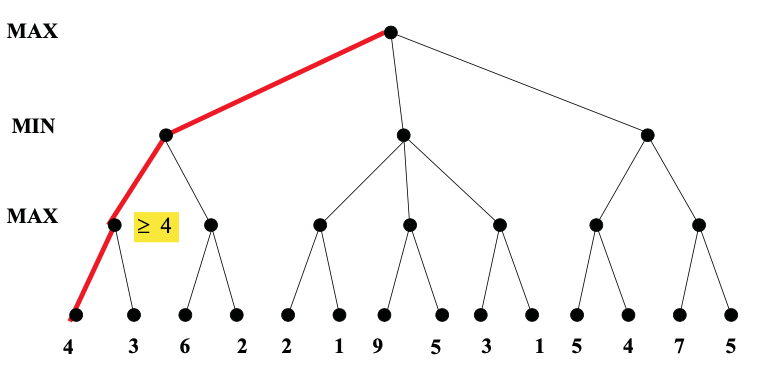
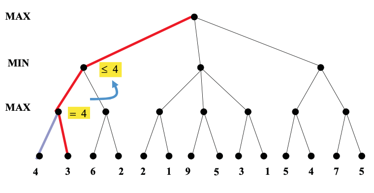
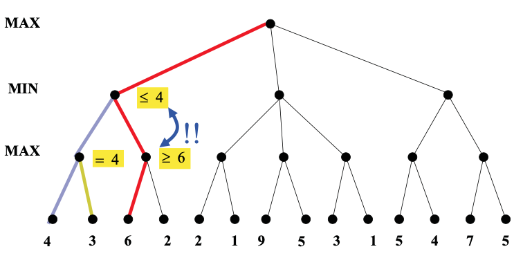
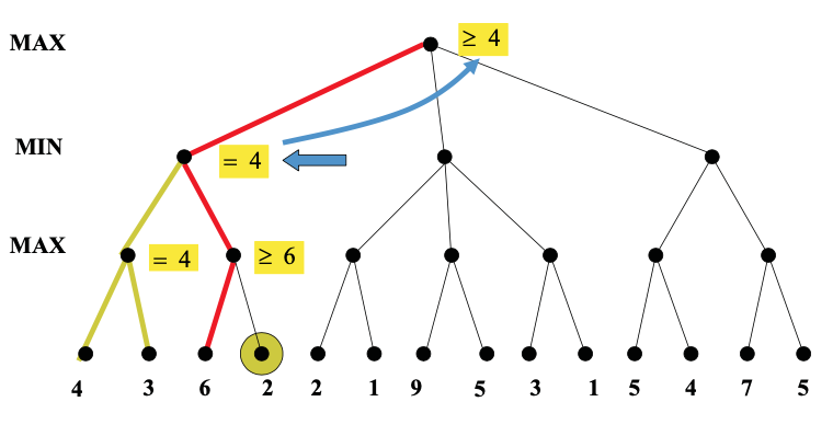
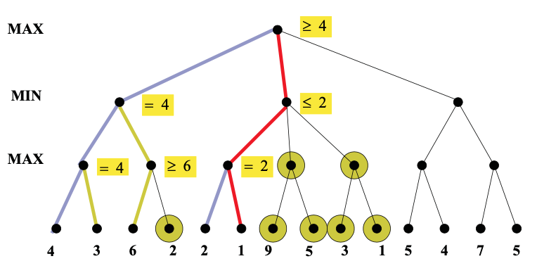
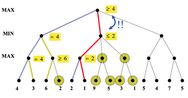
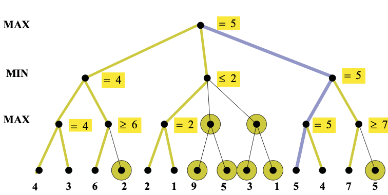
As you can see from this example, this strategy can greatly reduce the amount of the tree we have to explore. Remember that we're building the game tree dynamically as we do depth-first search, so "don't have to explore" means that we never even allocate those nodes of the tree.
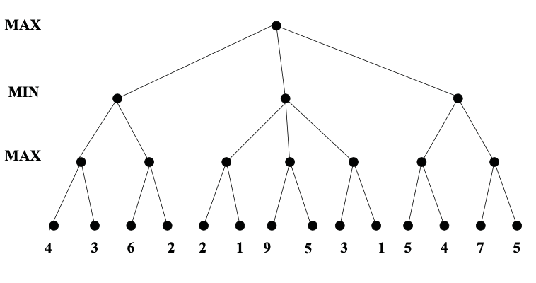
For further examples, see this alpha-beta pruning demo from Pascal Schärli.
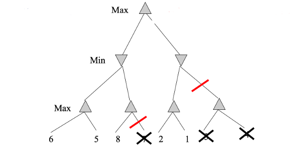
That the left-to-right order of nodes matters to the performance of alpha-beta pruning. Remember that the tree is built dynamically, so this left-to-right ordering is determined by the order in which we consider the various possible actions (moves in the game). So the node order is something we can potentially control.
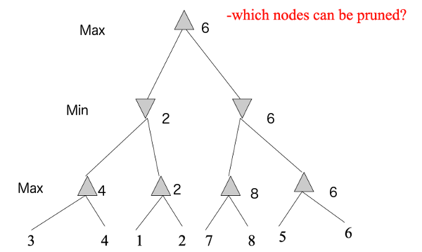
Consider this example (from Mitch Marcus (U. Penn), adapted from Rick Lathrop (USC)).

None of these nodes can be pruned by alpha-beta, because the best values are always on the righthand branch.
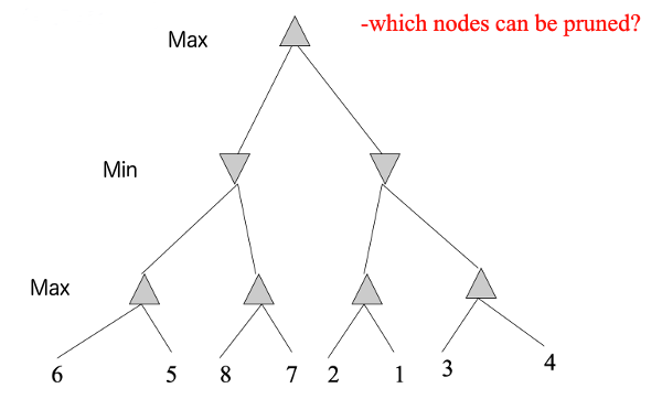
If we reverse the left-to-right order of the values, we can do considerable pruning:
Suppose that we have b moves in each game state (i.e. branching factor b), and our tree has height m. Then standard minimax examines \(O(b^m) \) nodes. If we visit the nodes in the optimal order, alpha-beta pruning will reduce the number of nodes searched to \(O(b^{m/2}) \). If we visit the nodes in random order, we'll examine \(O(b^{3m/4}) \) on average.
Obviously, we can't magically arrange to have the nodes in exactly the right order, because the whole point of this search is to find out what values we have at the bottom. However, heuristic ordering of actions can get close to the optimal \(O(b^{m/2})\) in practice. For example, a good heuristic order for chess examines possible moves in the following order:
Recall that our basic minimax search algorithm looks like this:
In order to discuss the details of alpha-beta pruning, we need to write detailed pseudocode for minimax. In building out our search tree, we create the children of a node n by taking an action, e.g. moving a piece in a chess game. Let's define:
Minimax is usually implemented using two mutually recursive functions, min-value and max-value. The input to min-value should be a min node and min-value returns the minimax value for that node. The function max-value does the same thing for an input max node.
max-value (node)
- if node is a leaf, return its value
- else
- rv = -inf
- for each action a
- childval = min-value(move(node,a))
- rv = max(rv, childval)
- return rv
min-value (node)
- if node is a leaf, return its value.
- else
- rv = +inf
- for each action a
- childval = max-value(move(node,a))
- rv = min(rv, childval)
- return rv
The above functions compute the value for the top node in the game tree. That will be convenient for discussing alpha-beta pruning. However, it's not actually what you'll do if you are implementing a game player. A game player needs his next move, not the value for the root node of the tree (aka the current game state). So our game playing code starts with a modified function at the top level which does this:
Choose-move(n)
- Create nodes for all children of n.
- Use min-value to compute the value for each child node.
- Pick the action corresponding to the child with the best value.
Detailed code for choose-move is essentially similar to max-value, except that it returns argmax rather than max.
To add alpha-beta pruning to our minimax code, we need two extra variables named (big surprise!) \(\alpha\) and \(\beta\). The algorithm passes \(\alpha\) and \(\beta\) downwards when doing depth-first search. We'll use \(\alpha\) and \(\beta\) to propagate information from earlier parts of our search to the path that we're currently exploring.
Suppose that our search is at some node n. There may be a number of paths leading from the root downwards to a leaf, via n. The "outcome" of a path is the value that it sends upwards to the root (which might not be the best value that arrives at the root).
The values of \(\alpha\) and \(\beta\) are based partly on values from descendents of the current node n. However, they are also based on values from already-explored nodes to the left of n. When nodes to the left of n have already found a better value for one of n's ancestors, we can stop exploring the descendents of n. The word "better" might translate into either larger or smaller, depending on whether the ancestor is a max or min node.
Suppose that v(n) is the value of our current node n (based on the children we have examined so far). If there's still a chance that the best path goes through n, we must have
\(\alpha \le v(n) \le \beta\)
As a node examines more and more of its children
We return prematurely if either of the following two situations holds:
Here's the pseudo-code for minimax with alpha-beta pruning. The changes from normal minimax are shown in red. Inside the inner loop for max-value, notice that rv gradually increases, as does alpha. The function returns prematurely if rv reaches beta.
max-value (node, alpha, beta )
- if node is a leaf, return its value.
- else
- rv = -inf
- for each action a
- childval = min-value(move(node,a), alpha, beta )
- rv = max(rv, childval)
- if rv >= beta, return rv # abandon this node as non-viable
- else alpha = max(alpha, rv)
- return rv
Similarly, inside the inner loop for min-value, rv gradually decreases and so does beta. The function returns prematurely if rv reaches alpha.
min-value (node, alpha, beta )
- if node is a leaf, return its value.
- else
- rv = +inf
- for each action a
- childval = max-value(move(node,a), alpha, beta)
- rv = min(rv, childval)
- if rv <= alpha, return rv # abandon this node as non-viable
- else beta = min(beta,rv)
- return rv
Yes, it's very easy to get parts of this algorithm backwards. We're not going to ask you to produce this level of detail on an exam. Concentrate on understanding what branches will be pruned, as shown in the previous lecture. But it's worth seeing the pseudocode briefly so that you can feel confident that alpha-beta pruning isn't complicated if you ever need to implement it.
A stochastic game is one in which some changes in game state are random, e.g. dice rolls, card games. That is to say, most board and card games. These can be modelled using game trees with three types of nodes
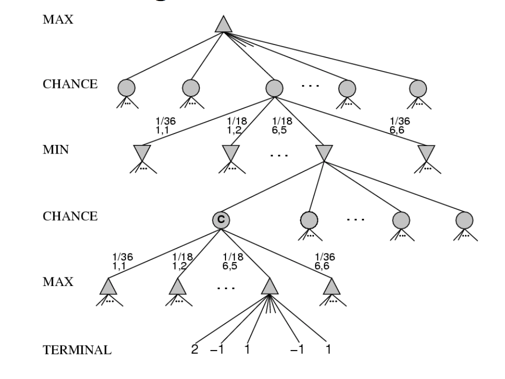
from Russell and Norvig
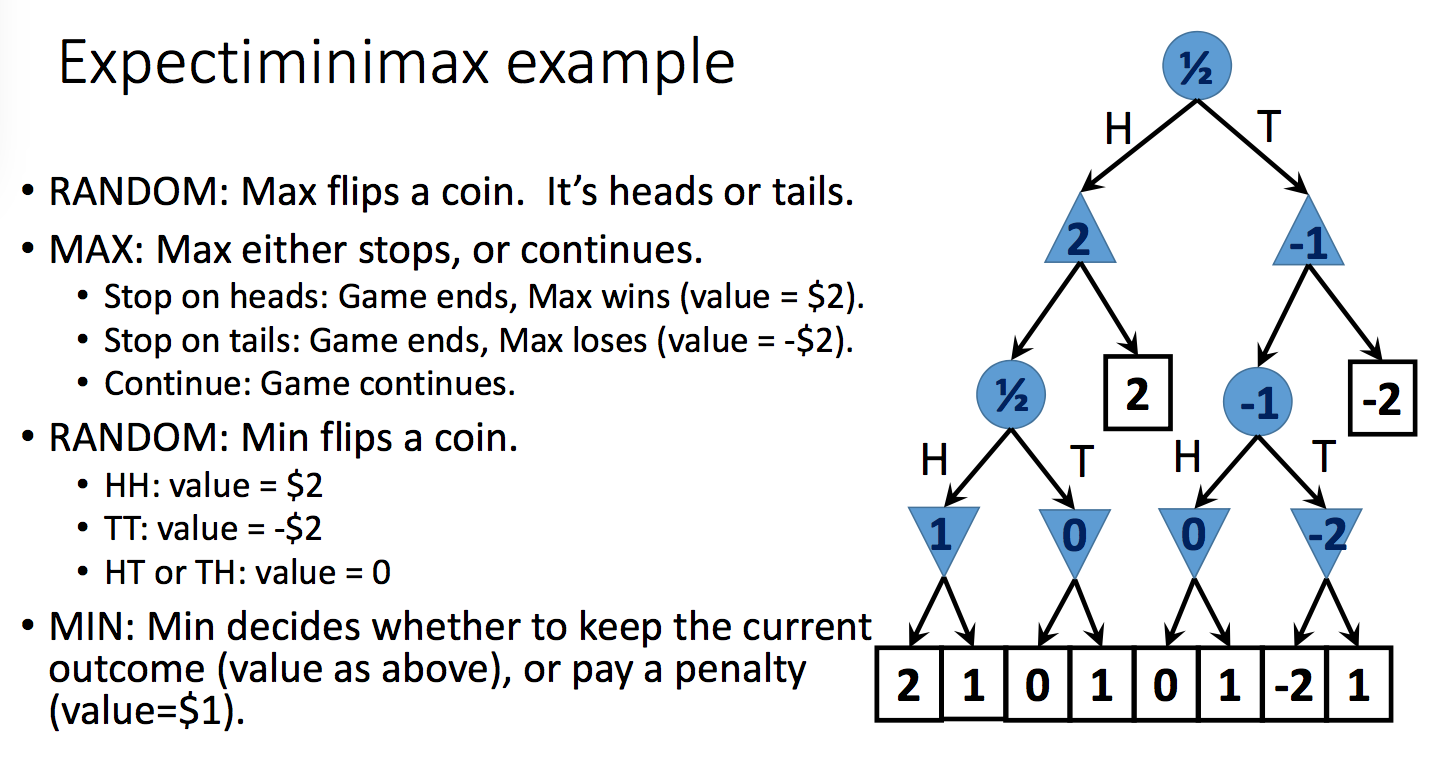
Expectiminimax is an extension of minimax for propagating values upwards in trees with chance nodes. Min and max nodes work as normally. For chance nodes, node value is the expected value over all its children.
That is, suppose the possible outcomes of a random action are \(s_1, s_2, ..., s_n\). Put each outcome in its own child node. Then the value for the parent node will be \( \sum_k P(s_k)v(s_k) \). The toy example below shows how this works:
 from Lana Lazebnik
This all works in theory. However, chance nodes add enough level to the tree and, in some cases (e.g. card games), they can have a high branching factor. So games involving random section (e.g. poker) can quickly become hard to solve by direct search.
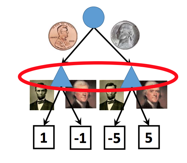
A related concept is imperfect information. In a game with imperfect information, there are parts of the game state that you can't observe, e.g. what's in the other player's hand. Again, typical of many common board and card games. We can also draw these as chance nodes, as in the example below (from Lana Lazebnik). Notice that Lincoln's face is on the penny and Jefferson's face is on the nickel.
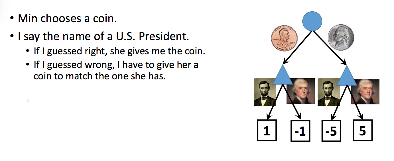
One way to model such a situation is to say that the agent is in one of several states:
In broad outline, this is similar to the standard trick in automata theory for modelling an NFA using a DFA whose states are sets of NFA states. The game playing program would then pick a common policy that will work for the whole set of possible states. For example, if you're playing once and can't afford to lose, you might pick the policy that minimizes your loss in the worst case. In the example above, this approach would pick Jefferson.
In a more complex situation, the group of states might share common features that could be leveraged to make a good decision. For example, suppose you are driving in a city and have gotten lost. You stop to ask for directions because you "have no idea" where you are. Actually, you probably do have some idea. If you're unsure of your city but can narrow it down to Illinois, you can ask for directions in English. If your possible cities are all in Quebec, you'd do this in French. Your group of alternative states shares a common geographic feature. This can be true for complex game states, e.g. you don't know their exact hand but it apparently contains some diamonds.
Alternatively, we could restructure the representation so that we have a stochastic chance node after our move, as in this picture:
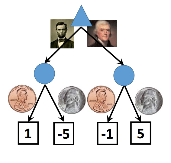
This is a good approach if you are playing the game repeatedly and have some theory of how likely the two coins are. If the two coins are equally likely, the corresponding expectiminimax analysis would compute the expected value for each of the two chance nodes (-2 for the left one, 2 for the right one). This again leads to a choice of Jefferson. However, in this case, the best choice will change depending on our theory of how likely the two types of coins are.
But what if our opponent is thinking ahead? How often would she actually choose to pick the penny vs. the nickel? Or, if she's picking randomly from a bag of coins, what percentage of the coins are really pennies?
>>> Question for the reader: what probability of penny vs. nickel would be required to change our best choice to Lincoln?
Game trees involving chance nodes can quickly become very large, restricting exhaustive search to a small lookahead in terms of mvoes. One method for getting the most out of limited search time is to randomly select trees. That is
This method limits to the correct node values as n gets large. In practice, we make n as large as resources allow and live with the resulting approximation error.
A similar approach can be used on deterministic games where the trees are too large for other reasons. That is
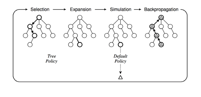
from C. Browne et al., A survey of Monte Carlo Tree Search Methods, 2012
Poker is a good example of a game with both a chance component and incomplete information. It is only recently that poker programs are competitive. CMU's Libratus system recently (2017) beat some of the best human players (GeekWire, CMU news).
Libratus uses three modules to handle three key tasks:
It used a vast amount of computing power: 600 of the 846 compute nodes in the "Bridges" supercomputer center. Based on the news articles, this would have 1 pentaflop, i.e. 5147 times as much processing power as a high-end laptop. And the memory was 195 Terabyes, i.e. 12,425 times as much as a high-end laptop. This is a good example of current state-of-the-art game programs requiring excessive amounts of computing resources, because game performance is so closely tied to the raw amount of search that can be done. However, improvements in hardware have moved many AI systems from a similar niche to eventual installation on everyday devices.
For a more theoretical (probably completmentary) approach, check out the CFR* Poker algorithm.
Another very recent development are programs that play Go extremely well. AlphaGo and its successor AlphaZero combine Monte Carlo tree search with neural networks that evaluate the goodness of board positions and estimate the probability of different choices of move. In 2016, AlphaGo beat Lee Se-dol, believed to be the top human player at the time. More recent versions work better and seem to be consistently capable of beating human players.
More details can be found in
In a recent news article, the BBC reported that Lee Se-dol quit because AI "cannot be defeated." However humans can still beat AI with the right strategy