The last few topics in this course cover specialized types of search. These were once major components of AI systems. They are are still worth knowing about because they still appear in the higher-level (more symbolic) parts of AI systems. We'll start by looking at constraint satisfaction problems.
Remember that a queen in chess threatens another piece if there is a direct path between the two either horizontally, or vertically, or diagonally. In the n queens problem, we have to place n queens on a n by n board so that no queen threatens another. Here is a solution for n=8:
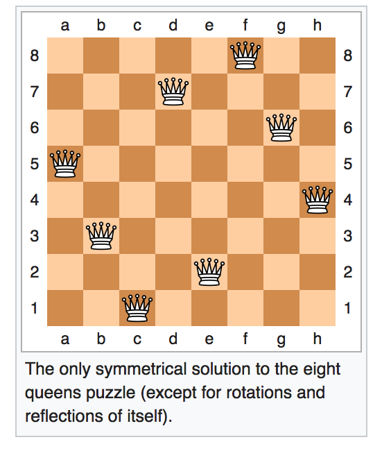
From Wikipedia
Since each column must contain exactly one queen, we can model this as follows
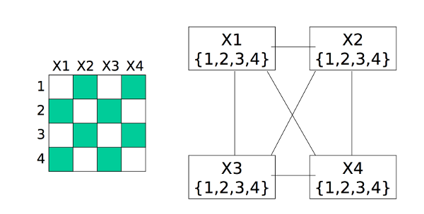
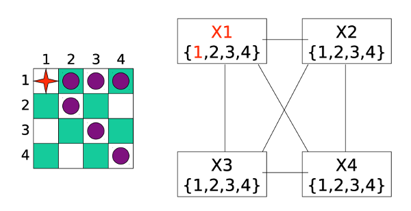
We can visualize this as a graph in which each variable is a node and edges link variables involved in binary constraints. To make something easy to draw, consider the 4-queens problem shown below. X1 is a variable representing a column. Its possible values {1,2,3,4} are the row to place the queen in. X2 has a similar set of possible values. X1 and X2 are linked by a constraint arc because we need to ensure that the queens in these two columns aren't in the same row or diagonal.
from Bonnie
Dorr, U. Maryland
(via Mitch Marcus at U. Penn).
A constraint-satisfaction problem (CSP) consists of
In many examples, all variables have the same set of allowed values. But there are problems where different variables may have different possible values.
Need to find a complete assignment (one value for each variable) that satisfies all the constraints
In basic search problems, we are explicitly given a goal (or perhaps a small set of goals) and need to find a path to it. In a constraint-satisfaction problem, we're given only a description of what constraints a goal state must satisfy. Our problem is to find a goal state that satisfies these constraints. We do end up finding a path to this goal, but the path is only temporary scaffolding.

From
Wikipedia
Viewed as a CSP problem
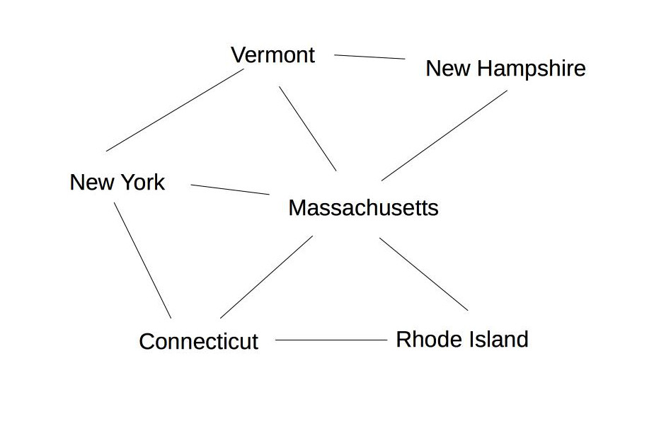
Pictured as a constraint graph, the states/countries are nodes, and edges connect adjacent states. A small example is shown below. Theoretical work on this topic is found mostly under the keyword "graph coloring." Applications of graph coloring include register allocation, final exam scheduling.
The "4 color Theorem" states that any planar map can be colored with only four colors. It was proved at U. Illinois in 1976 by Kenneth Appel and Wolfgang Haken. It required a computer program to check almost 2000 special cases. This computer-assisted proof was controversial at the time, but became accepted after the computerized search had been replicated a couple times.
Notice that graph coloring is NP complete. We don't know for sure if NP problems require polynomial or exponential time, but we suspect they require exponential time. However, many practical applications can exploit domain-specific heuristics (e.g. linear scan for register allocation) or loopholes (e.g. ok to have small conflicts in final exams) to produce fast approximate algorithms.
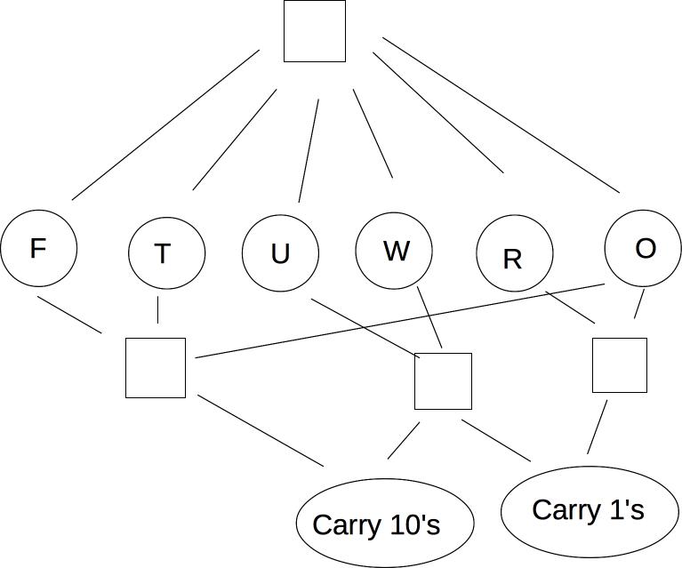
Cryptarithmetic is another classic CSP problem. Here's an example:
             T W O
           + T W O
         ---------
         = F O U R
We can make this into a CSP model as follows:
"Addition works as intended" can be made concrete with these equations, where C_1 and C_10 are the carry values.
     O + O = R + 10 * C_1
     W + W + C_1 = U + 10*C_10
     T + T + C_10 = O + 10*F
"All different" and the equational constraints involve multiple variables. Usually best to keep them in that form, rather than converting to binary. We can visualize this using a slightly different type of graph with some extra nodes:
from
Wikipedia
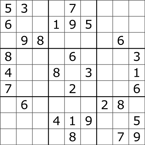
Sudoku can be modelled as a CSP problem,
We can also use this framework to model scheduling problems, e.g. planning timing and sequence of operations in factory assembly.
There are two basic approaches to solving constraint satisfaction problems: hill climbing and backtracking search. CSP problems may include multi-variate constraints. E.g. sudoku requires that there be no duplicate values within each row/column/block. For this class, we'll stick to constraints involving two variables.
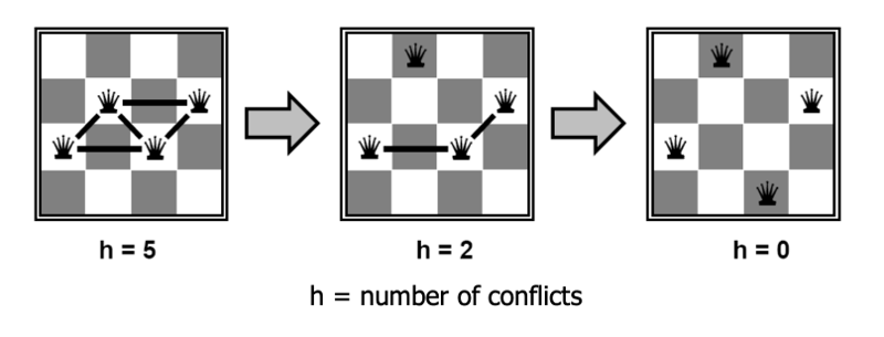
In the hill-climbing approach, we pick a full set of variable assignments, then try to tweak it into a legal solution. The initial choice would be random if we're starting from scratch. Or we could initial with a solution to a similar problem. E.g. we might initialize this term's course scheduling problem with last term's schedule. At each step, our draft solution will have some constraints that are still violated. We change the value of one variable to try to reduce the number of conflicts as much as possible. (If there are several options, pick one randomly.) In the following example, this strategy works well:
from Lana Lazebnik, Fall 2017
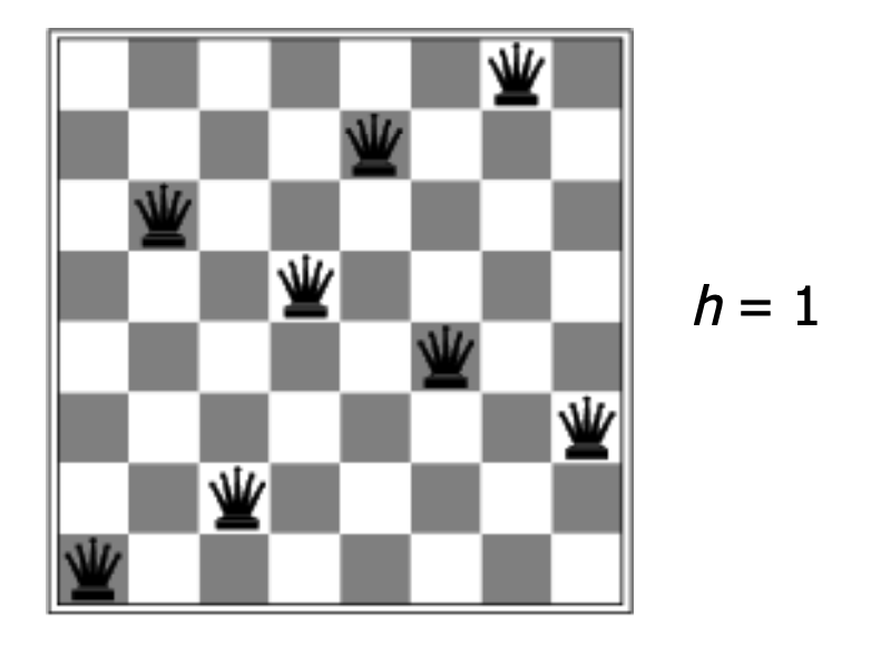
Hill climbing can be very effective on certain problems, and people frequently use it to solve complicated constraint satisfaction problems, e.g. scheduling classes or final exams. However, this method can get stuck in local optima. For example, the following configuration for 8 Queens has a single constraint violation, but no adjustment of a single piece will reduce the number of violations to zero.
from Lana Lazebnik, Fall 2017
To avoid being stuck in local optima, hill-climbing algorithms often add some randomization:
The other basic approach to a constraint satisfaction problem is to choose variable values one at a time, undoing assignments ("backtracking") when we discover that our current set of assignments can't work. Specifically, we set up search as follows:
CSP search has some special properties which will affect our choice of search method. If our problem has n variables, then all solutions are n steps away. So DFS is a good choice for our search algorithm.
We can use a very stripped down DFS implementation, without explicit loop detection. This can be made to use only a very small amount of memory. In this type of AI context, DFS is often called "backtracking search" because it spends much of its time getting blocked and retreating back up the search tree to try other options.
A variety of heuristics can be used to speed up backtracking search. Let's start by looking at when to detect that our path is failing and we need to backtrack.
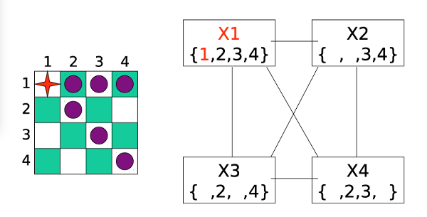
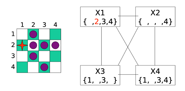
Here is a little demo of forward checking, from Bonnie Dorr, U. Maryland, via Mitch Marcus at U. Penn. We start with each variable x having a full list of possible values D(x) and no assignments.
First, we assign a value to the first variable. The purple cells show which other assignments are now problematic.
Forward checking now removes conflicting values from each list D(x).
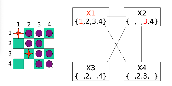
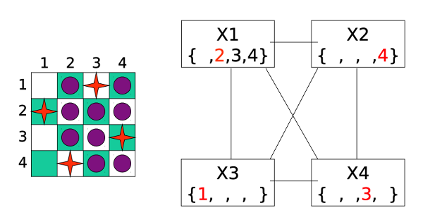
We now pick a value for our second variable.
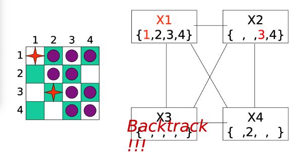
However, when we do forward checking, we discover that variable X3 has no possible values left. So we have to backtrack and undo the most recent assignment (to X2).
After some more assignments and backtracking, we end up giving up on X1=1 and moving on to exploring X1=2.
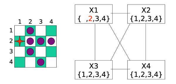
Forward checking reduces the sets of possible values to this:
After a few more steps of assignments and forward checking, we reach a full solution to the problem:
In the previous example, we tried variables in numerical order, i.e. how they came to us in the problem statement. When solving more complex problems, it can be important to use a smarter selection method. For example:
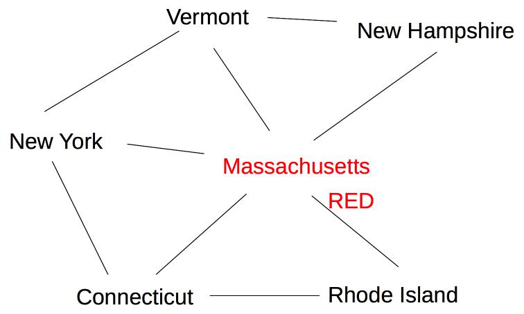
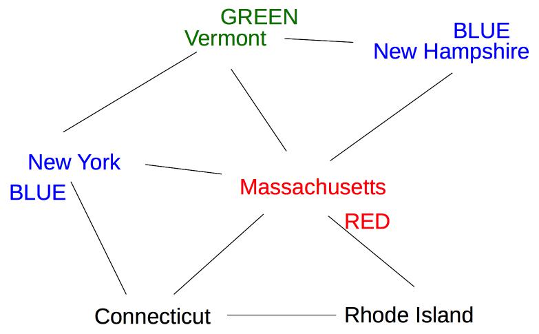
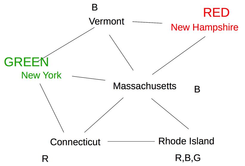
Suppose we are coloring the following graph with 3 colors (red, green, blue).
All states have three possible color values, so we use heuristic (b) and pick a color for Massachusetts:
The five remaining states are still tied on (a), so we use heuristic (b) to pick one of the states with three neighbors (Vermont):
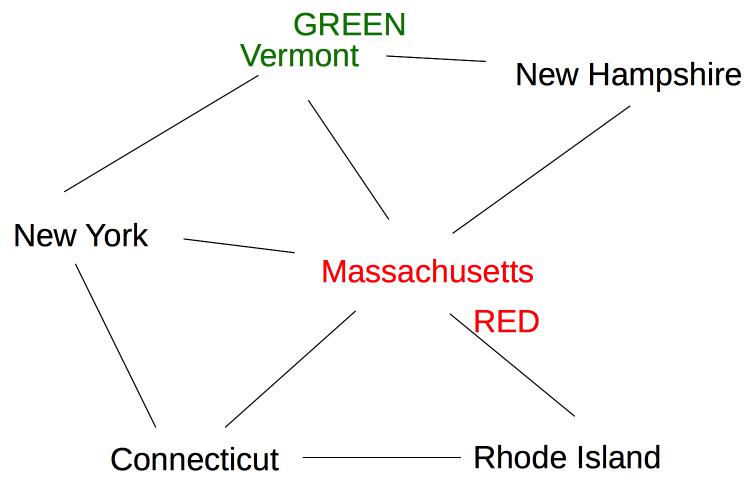
Now two states (New York and New Hampshire) have only one possible color value (blue), so we color one of them next:
Once we've chosen a variable, we can be smart about the order in which we explore its values. A good heuristic is:
For example, suppose we're trying to pick a value for the lower left node in the graph below. We should try Green first, because it leaves two color options open for the lower right node.
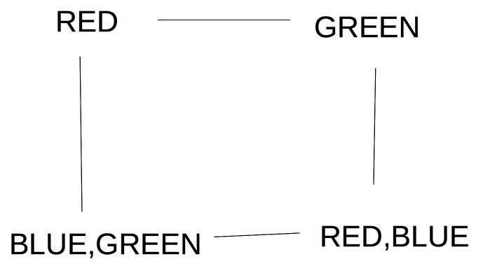
If this preferred choice doesn't work out, then we'll back up and try the other choice (Blue).
Constraint solving code should be designed to exploit any internal symmetries in the problem. For example, the map coloring problem doesn't care which color is which. So it doesn't matter which value we pick for the first variable (sometimes also some later choices). Similarly, there aren't really four distinct choices for the first column of n-queens, because reflecting the board vertically (or horizontally) doesn't change the essential form of the solution.
Here's our curent algorithm for solving a constraint satisfaction problem.
For each variable X, maintain set D(X) containing all possible values for X.
Run DFS. At each search step:
- Pick a value for one variable. (Back up if no choices are available.)
- Forward checking: prune all the sets D(X) to remove violations of constraints
Until we reach a state with a complete legal solution.
When we assign a value to variable X, forward checking only checks variables that share a constraint with X, i.e. are adjacent in the constraint graph. This is helpful, but we can do more to exploit the constraints. Constraint propagation works its way outwards from X's neighbors to their neighbors, continuing until it runs out of nodes that need to be updated.
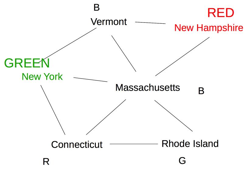
Suppose we are coloring the same state graph with {Red,Green,Blue} and we decide to first color New Hampshire red:
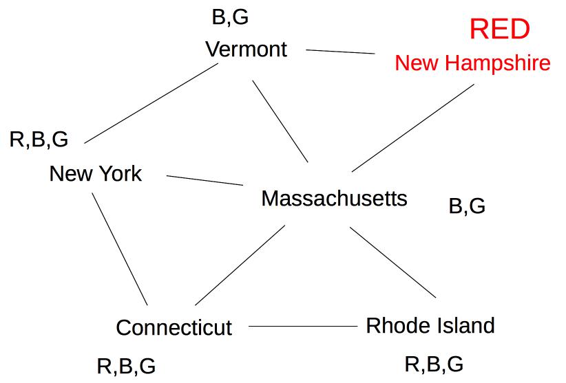
Forward checking then removes Red from Vermont and Massachusetts. Suppose we now color New York Green. Forward checking removes Green from its immediate neighbors, giving us this:
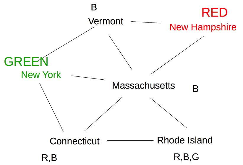
At this point, forward checking stops. Constraint propagation continues. Since the value set for Massachusetts has been reduced, we need to check its neighbors. Connecticut also needs to be updated. Since the only possible label for Massachusetts is blue, Connecticut can't have label blue.
Rhode Island is adjacent to Massachusetts and Connecticut, so its options need to be updated:
Finally, Vermont is also neighbor of Massachusetts, so we need to update its options.
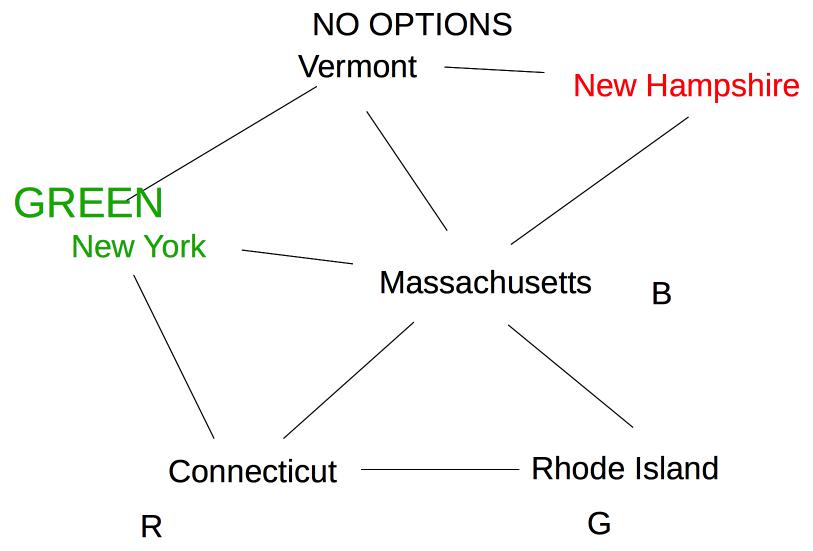
Oops! Vermont is left with no possible values, so we must backtrack to our last decision point (coloring New York Green).
The exact sequence of updates depends on the order in which we happen to have stored our nodes. However, constraint propagation typically makes major reductions in the number of options to be explored, and allows us to figure out early that we need to backtrack.
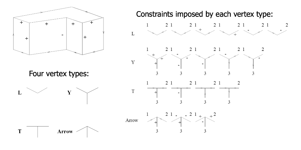
Constraint propagation was developed by David Waltz in the early 1970's for the Shakey project (e.g. see David Waltz's 1972 thesis). The original task was to take a wireframe image of blocks and decorate each edge with a labels indicating its type. Object boundaries are indicated by arrows, which need to point clockwise around the bounary. Plus and minus signs mark internal edges that are convex and concave.
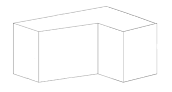
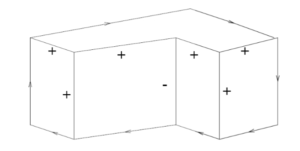
In this problem, the constraints are provided by the vertices. Each vertex is classified into one of four types, based on the number of edges and their angles. For each type, there are only a small set of legal ways to label the incoming edges.
See this contemporary video of the labeller in action.
Because line labelling has strong local constraints, constraint propagation can sometimes nail down the exact solution without any search. A more typical situation is that we need to use a combination of backtracking search and constraint propagation. Constraint propagation can be added at either, or both, of the following places in our backtracking search:
It takes a bit of care to implement constraint propagation correctly. We'll look at the AC-3 algorithm, developed by David Waltz and Alan Mackworth (1977).
The constraint relationship between two variables ("some constraint relates the values of X and Y") is symmetric. For this algorithm, however, we will treat constraints between variables ("arcs") as ordered pairs. So the pair (X,Y) will represent contraint flowing from Y to X.
The function Revise(X,Y) prunes values from D(X) that are inconsistent with what's currently in D(Y).
The main datastructure in AC-3 is a queue of pairs ("arcs") that still need attention.
Given these definitions, AC-3 works like this:
Initialize queue. Two options
- all constraint arcs in problem [for starting up a new CSP search]
- all arcs (X,Y) where Y's value was just set [for use during CSP search]
Loop:
- Remove (X,Y) from queue. Call Revise(X,Y).
- If D(X) has become empty, halt returning a value that forces main algorithm to backtrack.
- If D(X) has been changed (but isn't empty), push all arcs (C,X) onto the queue. Exception: don't push (Y,X).
Stop when queue is empty
Near the end of AC-3, we push all arcs (C,X) onto the queue, but we don't push (Y,X). Why don't we need to push (Y,X)?
Do attempt to solve this yourself first. It will help you internalize the details of the AC-3 algorithm. Then have a look at the solution below.
See the CSPLib web page for more details and examples.
In the CSP lectures, I left the following question unanswered:
Near the end of AC-3, we push all arcs (C,X) onto the queue, but we don't push (Y,X). Why don't we need to push (Y,X)?
There's two cases. First (Y,X) might already be in the queue.
If (Y,X) is already in the queue, then we don't need to add it.
If (Y,X) is not already in the queue, then we've already checked (Y,X) at some point in the past. That check ensured that every value in D(Y) had a matching value in D(X). And, moreover, nothing has happened to D(X) since then, until what we did in the current step of AC-3.
The current step of AC-3 is repairing a problem caused by D(Y) having become smaller. So the situation at the start of our step is that:
Our call to Revise(X,Y) removes that second group of unmatched values. But it doesn't do anything to the first group of values with matches, because the constraint is symmetric. So, after our call to Revise(X,Y), D(X) and D(Y) are now completely consistent with one another.