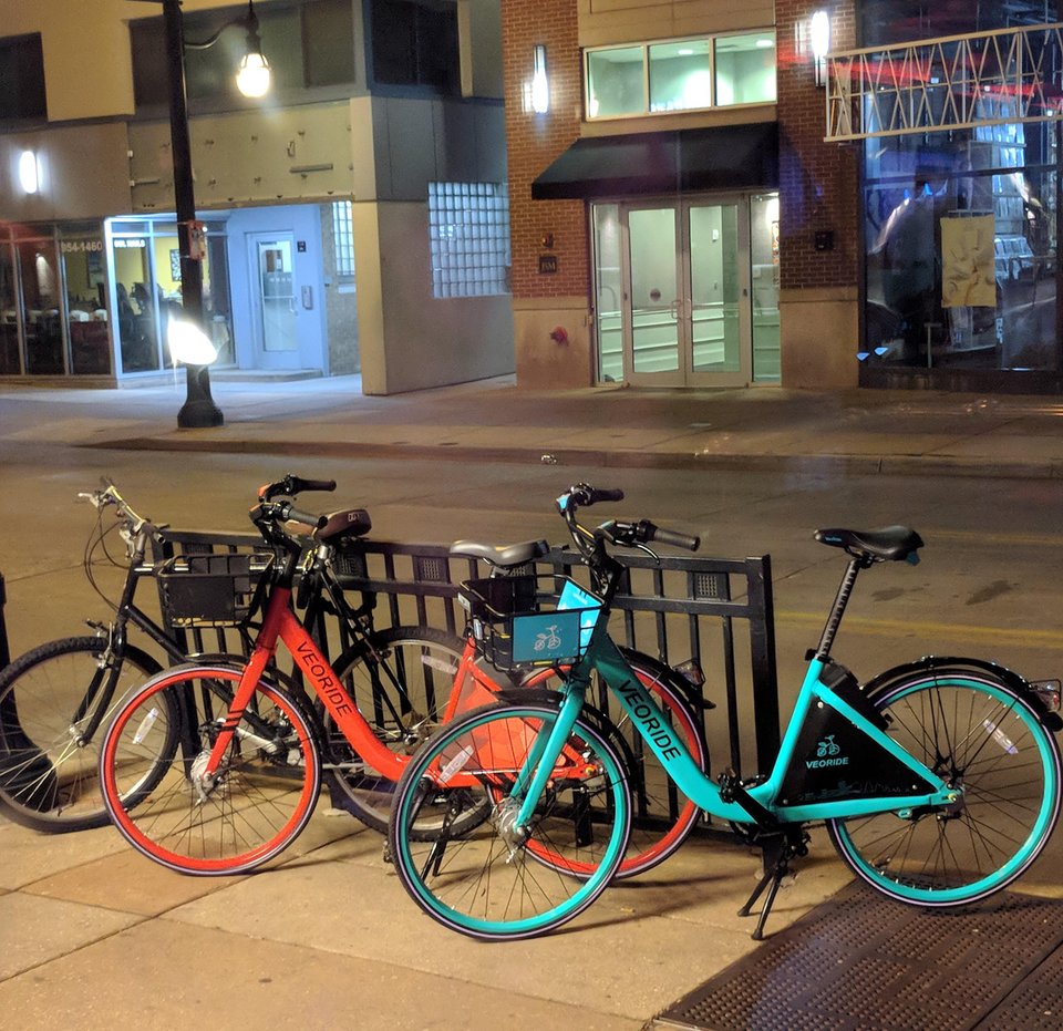
 Red and teal veoride bikes from /u/civicsquid reddit post
Suppose we are building a more complete bike recognition system. It might observe (e.g. with its camera) features like:
How do we combine these types of evidence into one decision about whether the bike is a veoride?
As we saw earlier, a large number of parameters would be required to model all of the \(2^n\) interactions between n variables. The Naive Bayes algorithm reduces the number of parameters to O(n) by making assumptions about how the variables interact,
Remember that two events A and B are independent iff
P(A,B) = P(A) * P(B)
Sadly, independence rarely holds. A more useful notion is conditional independence. That is, are two variables independent when we're in some limited context. Formally, two events A and B are conditionally independent given event C if and only if
P(A, B | C) = P(A|C) * P(B|C)
Conditional independence is also unlikely to hold exactly, but it is a sensible approximation in many modelling problems. For example, having a music stand is highly correlated with owning a violin. However, we may be able to treat the two as independent (without too much modelling error) in the context where the owner is known to be a musician.
The definiton of conditional independence is equivalent to either of the following equations:
P(A | B,C) = P(A | C)
P(B | A,C) = P(B | C)
It's a useful exercise to prove that this is true, because it will help you become familiar with the definitions and notation.
Suppose we're observing two types of evidence A and B related to cause C. So we have
P(C | A,B) \( \propto \) P(A,B | C) * P(C)
Suppose that A and B are conditionally independent given C. Then
P(A, B | C) = P(A|C) * P(B|C)
Substituting, we get
P(C | A,B) \( \propto \) P(A|C) * P(B|C) * P(C)
This model generalizes in the obvious way when we have more than two types of evidence to observe. Suppose our cause C has n types of evidence, i.e. random variables \( E_1,...,E_n \). Then we have
\( P(C | E_1,...E_n) \ \propto\ P(E_1|C) * ....* P(E_n|C) * P(C) \ = \ P(C) * \prod_{k=1}^n P(E_k|C) \)
So we can estimate the relationship to the cause separately for each type of evidence, then combine these pieces of information to get our MAP estimate. This means we don't have to estimate (i.e. from observational data) as many numbers. For n variables, a naive Bayes model has only O(n) parameters to estimate, whereas the full joint distribution has \(2^n\) parameters.
The following word clouds show which words (content words only) were said most by Clinton and Trump in their first debate:
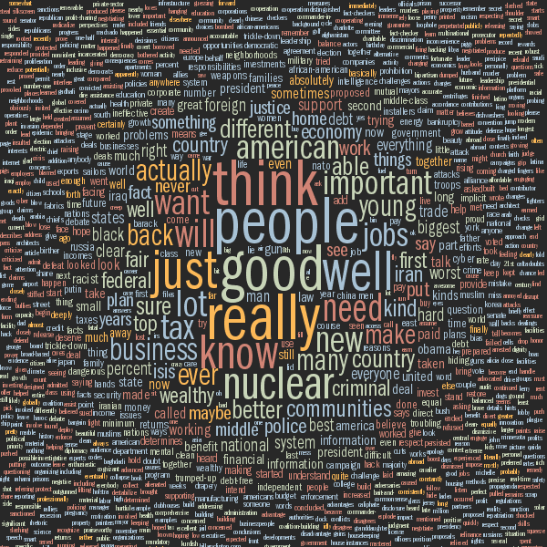
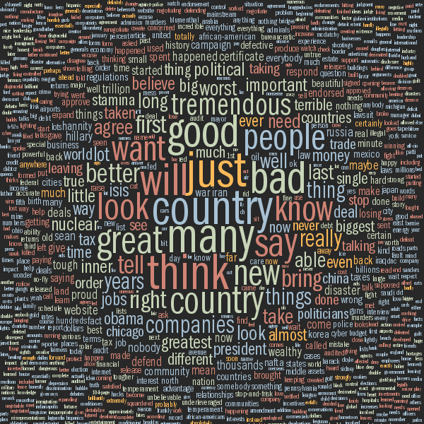
Word cloud visualizations of word frequency (content-words only) from the first Clinton-Trump debate. From Martin Krzywinski's Word Analysis of 2016 Presidential Debates. (Left is Clinton.)
The basic task is
Input: a collection of objects of several types
Output: correct type label for each object
In practice, this means
Input: a collection of objects of several types
Extract features from each object
Output: Use the features to label each object with its correct type
For example, we might wish to take a collection of documents (i.e. text files) and classify each document by type. For example:
We might use features such as words, partial words, and/or short sequences of words.
Let's look at the British vs. American classification task. Certain words are characteristic of one dialect or the other. For example
See this list of British and American words. The word "boffin" differs from "egghead" because it can be modified to make a wide range of derived words like "boffinry" and "astroboffin". Dialects have special words for local foods, e.g. the South African English words "biltong," "walkie-talkie," "bunny chow."
Bag of words model: We can use the individual words as features.
A bag of words model determines the class of a document based on how frequently each individual word occurs. It ignores the order in which words occur, which ones occur together, etc. So it will miss some details, e.g. the difference between "poisonous" and "not poisonous,"
Consider this sentence
The big cat saw the small cat.
It contains two pairs of repeated words. For example, \(W_3\) is "cat" and \(W_7\) is also "cat". Our estimation process will consider the two copies of "cat" separately
Jargon:
So our example sentence has seven tokens drawn from five types.
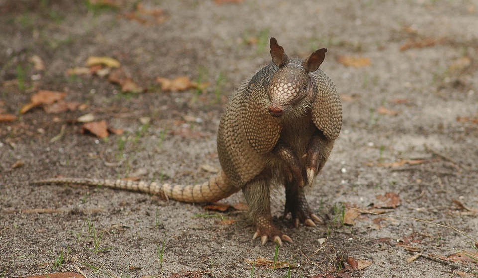
Armadillo (picture from Prairie Rivers Network)
Classification algorithms frequently ignore very frequent and very rare words. Very frequent words ("stop words") often convey very little information about the topic. So they are typically deleted before doing a bag of words analysis.
Stop words in text documents are typically function words, such as "the", "a", "you", or "in". In transcribed speech, we also see
However, whether to ignore stop words depends on the task. Stop words can provide useful information about the speaker's mental state, relation to the listener, etc. See James Pennebaker "The secret life of pronouns".
Rare words include words for uncommon concepts (e.g. armadillo), proper names, foreign words, obsolete words (e.g. abaft), numbers (e.g. 61801), and simple mistakes (e.g. "Computer Silence"). Words that occur only one (hapax legomena) often represent a large fraction (e.g. 30%) of the word types in a dataset. Rare words cause two problems
Rare words may be deleted before analyzing a document. More often, all rare words are mapped into a single placeholder value (e.g. UNK). This allows us to treat them all as a single item, with a reasonable probability of being observed.
Suppose that cause C produces n observable effects \( E_1,...,E_n \). Then our Naive Bayes model calculates the MAP estimate as
\( P(C | E_1,...E_n) \ \propto\ P(E_1|C) * ....* P(E_n|C) * P(C) \ = \ P(C) * \prod_{k=1}^n P(E_k|C) \)
Let's map this idea over to our Bag of Words model of text classification. Suppose our input document contains the string of words \( W_1, ..., W_n \). So \(W_k\) is the word token at position k. Suppose that \(P(W_k)\) is the probability of the corresponding word type.
To classify the document, naive Bayes compares these two values
\(P(\text{UK} | W_1, \ldots, W_n) \ \propto\ P(\text{UK}) * \prod_{k=1}^n P(W_k | \text{UK} ) \)
\( P(\text{US} | W_1, \ldots, W_n) \ \propto\ P(\text{US}) * \prod_{k=1}^n P(W_k | \text{US})\)
To do this, we need to estimate two types of parameters
Naive Bayes works quite well in practice, especially when coupled with a number of tricks that we'll see later. The Naive Bayes spam classifier SpamCop, by Patrick Pantel and Dekang Lin (1998) got down to a 4.33% error rate using bigrams and some other tweaks.
Suppose we have n word types, then creating our bag of words model requires estimating O(n) probabilities. This is much smaller than the full conditional probability table which has \(2^n\) entries. The big problem with too many parameters is having enough training data to estimate them reliably. (I said this last lecture but it deserves a repeat.)
A Quantitative Analysis of Lexical Differences Between Genders in Telephone Conversations Constantinos Boulis and Mari Ostendorf, ACL 2005
Fisher corpus of more than 16,000 transcribed telephone conversations (about 10 minutes each). Speakers were told what subject to discuss. Can we determine gender of the speaker from what words they used?
Words most useful for discriminating speaker's gender (i.e. used much more by men than women or vice versa)
This paper compares the accuracy of Naive Bayes to that of an SVM classifier, which is a more sophisticated classification technique.
The more sophisticated classifier makes an improvement, but not a dramatic one.
The high level classification model is simple, but a lot of details are required to get high quality results. Over the next three videos, we'll look at four aspects of this problem:
Training data: estimate the probability values we need for Naive Bayes
Development data: tuning algorithm details and parameters
Test data: final evalution (not always available to developer) or the data seen only when system is deployed
Training data only contains a sampling of possible inputs, hopefully typically but nowhere near exhaustive. So development and test data will contain items that weren't in the training data. E.g. the training data might focus on apples where the development data has more discussion of oranges. Development data is used to make sure the system isn't too sensitive to these differences. The developer typically tests the algorithm both on the training data (where it should do well) and the development data. The final test is on the test data.
Results of classification experiments are often summarized into a few key numbers. There is often an implicit assumption that the problem is asymmetrical: one of the two classes (e.g. Spam) is the target class that we're trying to identify.
| Labels from Algorithm | ||
|---|---|---|
| Spam | Not Spam | |
| Correct = Spam | True Positive (TP) | False Negative (FN) |
| Correct = Not Spam | False Positive (FP) | True Negative (TN) |
We can summarize performance using the rates at which errors occur:
Now, suppose we have a task that's well described as extracting a specific set of items from a larger input set. We can ask how well our output set contains all, and only, the desired items:
F1 is the harmonic mean of precision and recall. Both recall and precision need to be good to get a high F1 value.
For more details, see the Wikipedia page on recall and precision
We can also display a confusion matrix, showing how often each class is mislabelled as a different class. These usually appear when there are more than two class labels. They are most informative when there is some type of normalization, either in the original test data or in constructing the table. So in the table below, each row sums to 100. This makes it easy to see that the algorithm is producing label A more often than it should, and label C less often.
| Labels from Algorithm | |||
|---|---|---|---|
| A | B | C | |
| Correct = A | 95 | 0 | 5 |
| Correct = B | 15 | 83 | 2 |
| Correct = C | 18 | 22 | 60 |
We're now going to look at details required to make this classification algorithm work well.
Be aware that we're now talking about tweaks that might help for one application and hurt performance for another. "Your mileage may vary."
For a typical example of the picky detail involved in this data processing, see the method's section from the word cloud example in the previous lecture.
Our first job is to produce a clean string of words, suitable for use in the classifier. Suppose we're dealing with a language like English. Then we would need to
This process is called tokenization. Format features such as punctuation and capitalization may be helpful or harmful, depending on the task. E.g. it may be helpful to know that "Bird" is different from "bird," because the former might be a proper name. But perhaps we'd like to convert "Bird" to "CAP bird" to make its structure explicit. Similarly, "tyre" vs. "tire" might be a distraction or an important cue for distinguishing US from UK English. So "normalize" may either involve throwing away the information or converting it into a format that's easier to process.
After that, it often helps to normalize the form of each word using a process called stemming.
Stemming converts inflected forms of a word to a single standardized form. It removes prefixes and suffixes, leaving only the content part of the word (its "stem"). For example
       help, helping, helpful --->  help
       happy, happiness --> happi
Output is not always an actual word.
Stemmers are surprisingly old technology.
Porter made modest revisions to his stemmer over the years. But the version found in nltk (a currently popular natural language toolkit) is still very similar to the original 1980 algorithm.
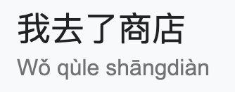
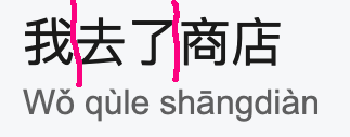
English has relatively short words, with convenient spaces between them. Tokenization requires slightly different steps for languages with longer words or different writing system. For example, Chinese writing does not put spaces between words. So "I went to the store" is written as a string of characters, each representing one syllable (below). So programs processing Chinese text typically run a "word segmenter" that groups adjacent characters (usually 2-3) into a word.
In German, we have the opposite problem: long words. So we might divide words like "Wintermantel" into "winter" (winter) and "mantel" (coat).
In either case, the output tokens should usually form coherent units, whose meaning cannot easily be predicted from smaller pieces.
The Bag of Words model uses individual words as features, ignoring the order in which they appeared. Text classification is often improved by using pairs of words (bigrams) as features. Some applications (notably speech recognition) use trigrams (triples of words) or even longer n-grams. E.g. "Tony the Tiger" conveys much more topic information than either "Tony" or "tiger". In the Boulis and Ostendorf study of gender classification bigram features proved significantly significantly more powerful.
For n words, there are \(n^2\) possible bigrams. But our amount of training data stays the same. So the training data is even less adequate for bigrams than it was for single words.
Recall our document classification problem. Our input document is a string of words (perhaps not all identical) \( W_1, ..., W_n \)
Suppose that we have cleaned up our words, as discussed in the last video and now we're trying to label input documents as either CLA or CLB. To classify the document, our naive Bayes, bag of words model, compares these two values:
Two classes \(C_1\) and \(C_2\).
\( P(C_1) * \prod_{k=1}^n P(W_k | C_1 ) \)
\( P(C_2) * \prod_{k=1}^n P(W_k | C_2)\)
We need to estimate the parameters \(P(W | C_1)\) and \(P(W | C_2)\) for each word type W.
Now, let's look at estimating the probabilities. Suppose that we have a set of documents from a particular class C (e.g. CLA English) and suppose that W is a word type. We can define:
count(W) = number of times W occurs in the documents
n = number of total words in the documents
A naive estimate of P(W|C) would be \(P(W | \text{C}) = \frac{\text{count}(W)}{n}\). This is not a stupid estimate, but a few adjustments will make it more accurate.
The probability of most words is very small. For example, the word "Markov" is uncommon outside technical discussions. (It was mistranscribed as "mark off" in the original Switchboard corpus.) Worse, our estimate for P(W|C) is the product of many small numbers. Our estimation process can produce numbers too small for standard floating point storage.
To avoid numerical problems, researchers typically convert all probabilities to logs. That is, our naive Bayes algorithm will be maximizing
\(\log(P(\text{C} | W_1,\ldots W_k))\ \ \propto \ \ \log(P(\text{C})) + \sum_{k=1}^n \log(P(W_k | \text{C}) ) \)
Notice that when we do the log transform, we need to replace multiplication with addition.
Recall that we train on one set of documents and then test on a different set of documents. For example, in the Boulis and Ostendorf gender classifcation experiment, there were about 14M words of training data and about 3M words of test data.
Training data doesn't contain all words of English and is too small to get a representative sampling of the words it contains. So for uncommon words:
Zeroes destroy the Naive Bayes algorithm. Suppose there is a zero on each side of the comparison. Then we're comparing zero to zero, although the other numbers may give us considerable information about the merits of the two outputs.
Smoothing assigns non-zero probabiities to unseen words. Since all probabilities have to add up to 1, this means we need to reduce the estimated probabilities of the words we have seen. Think of a probability distribution as being composed of stuff, so there is a certain amount of "probability mass" assigned to each word. Smoothing moves mass from the seen words to the unseen words.
Questions:
Some unseen words might be more likely than others, e.g. if it looks like a legit English word (e.g. boffin) it might be more likely than something using non-English characters (e.g. bête).
Smoothing is critical to the success of many algorithms, but current smoothing methods are witchcraft. We don't fully understand how to model the (large) set of words that haven't been seen yet, and how often different types might be expected to appear. Popular standard methods work well in practice but their theoretical underpinnings are suspect.
Laplace smoothing is a simple technique for addressing the problem:
All unseen words are represented by a single word UNK. So the probability of UNK should represent all of these words collectively.
n = number of words in our Class C training data
count(W) = number of times W appeared in Class C training data
To add some probability mass to UNK, we increase all of our estimates by \( \alpha \), where \(\alpha\) is a positive tuning constant, usually (but not always) no larger than 1. So our probabilities for UNK and for some other word W are:
P(UNK | C) = \(\alpha \over n\)
P(W | C) = \({count(W) + \alpha} \over n\)
This isn't quite right, because probabilities need to add up to 1. So we revise the denominators to make this be the case. Our final estimates of the probabilities are
V = number of word TYPES seen in training data
P(UNK | C) = \( \frac {\alpha}{ n + \alpha(V+1)} \)
P(W | C) = \( \frac {\text{count}(W) + \alpha}{ n + \alpha(V+1)} \)
When implementing Naive Bayes, notice that smoothing should be done separately for each class of document. For example, suppose you are classifying documents as UK vs. US English. Then Laplace smoothing for the UK English n and V would be the number of word tokens and word types seen in UK training data.
Performance of Laplace smoothing
A technique called deleted estimation (due to Jelinek and Mercer) can be used to directly measure these estimation errors.
Let's empirically map out how much counts change between two samples of text from the same source. So we divide our training data into two halves 1 and 2. Here's the table of word counts:
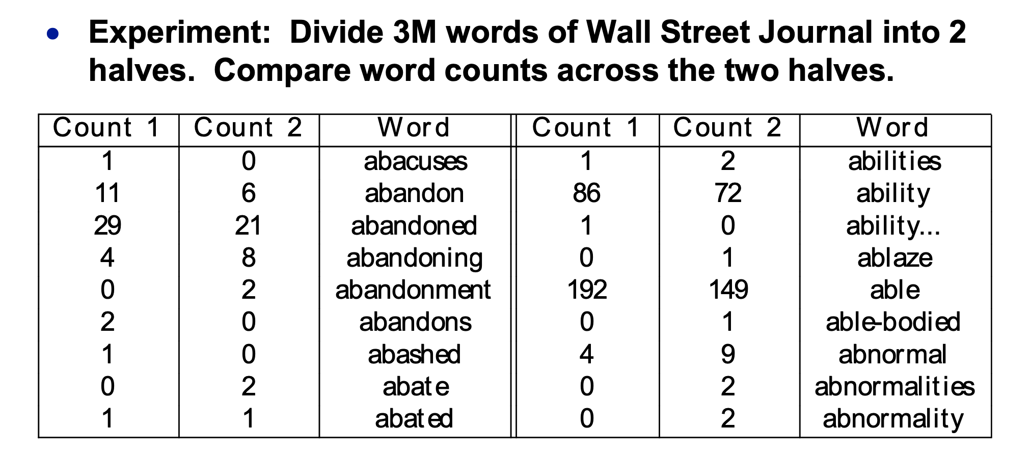 (from Mark Liberman via Mitch Marcus)
Now, let's pick a specific count r in the first half. Suppose that \(W_1,...,W_n\) are the words that occur r times in the first half. We can estimate the corrected count for this group of words as the average of their counts in the second half. Specifically, suppose that \(C(W_k)\) is the count of \(W_k\) in the SECOND half of the dataset. Then
Corr(r) = \(\frac{\sum_{k=1}^n C(W_k)}{n}\)
Corr(r) is a corrected count value that predicts future data more accurately.
This gives us the following correction table:
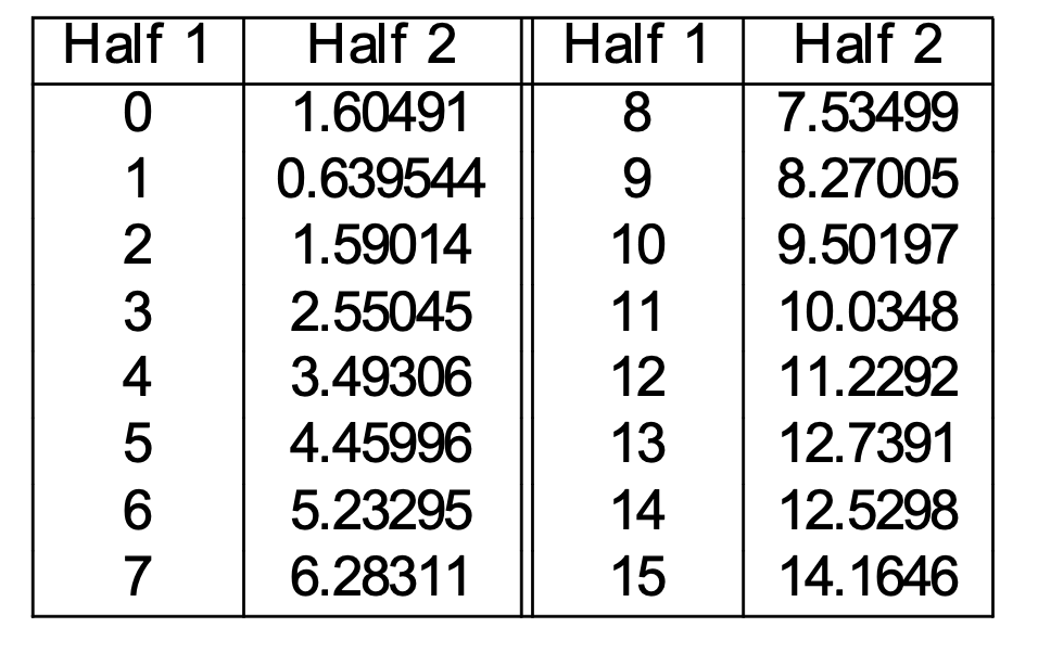
(from Mark Liberman via Mitch Marcus)
Finally, let's make the estimate symmetrical. Let's assume for simplicity that both halves contain the same number of words (at least approximately). Then compute
Corr(r) as above
Corr'(r) reversing the roles of the two datasets
\( {\text{Corr}(r) +\text{Corr}'(r)} \over 2\) estimate of the true count for a word with observed count r
And now we can compute the probabilities of individual words based on these corrected counts. These corrected estimates still have biases, but not as bad as the original ones. The method assumes that our eventual test data will be very similar to our training data, which is not always true.
Effectiveness of techniques like this depends on how we split the training data in half. Text tends to stay on one topic for a while. For example, if we see "boffin," it's likely that we'll see a repeat of that word soon afterwards. Therefore
Because training data is sparse, smoothing is a major component of any algorithm that uses n-grams. For single words, smoothing assigns the same probability to all unseen words. However, n-grams have internal structure which we can exploit to compute better estimates.
Example: how often do we see "cat" vs. "armadillo" on local subreddit? Yes, an armadillo has been seen in Urbana. But mentions of cats are much more common. So we would expect "the angry cat" to be much more common than "the angry armadillo". So
Idea 1: If we haven't seen an ngram, guess its probability from the probabilites of its prefix (e.g. "the angry") and the last word ("armadillo").
Certain contexts allow many words, e.g. "Give me the ...". Other contexts strongly determine what goes in them, e.g. "scrambled" is very often followed by "eggs".
Idea 2: Guess that an unseen word is more likely in contexts where we've seen many different words.
There's a number of specific ways to implement these ideas, largely beyond the scope of this course.