
Shakey the robot (1966-72), from Wired Magazine
\(A^*\) search was developed around 1968 as part of the Shakey project at Stanford. It's still a critical component of many AI systems. The Shakey project ran from 1966 to 1972. Here's some videos showing Shakey in action.
Towards the end of the project, it was using a PDP-10 with about 800K bytes of RAM. The programs occupied 1.35M of disk space. This kind of memory starvation was typical of the time. For example, the guidance computer for Apollo 11 (first moon landing) in 1969 had only 70K bytes of storage.
Cost so far is a bad predictor of how quickly a route will reach a goal. If you play around with this search technique demo by Xueqiao Xu, you can see that BFS and UCS ("Dijkstra") search a widening circular space, most of which is in the direction opposite to the goal. When they assess states, they consider only distance from the starting position, but not the distance to reach the goal.
Key idea: combine distance so far with an estimate of the remaining distance to the goal.
Basic outline is the same as UCS. That is, three types of states
The frontier is stored in a priority queue, with states ordered by their distance g(s) from the start state. We also store the distance g(S) to each state and a backpointer along its best path from the goal.
At each step of the search, we extract the state S with lowest g value. For each of S's neighbors, we check if it has already been seen. If it's new, add it to the frontier. Whe we return to a previously-seen state S via a new, shorter path, we update the stored distance g(S), the backpointer for S, and S's position in the priority queue.
Search stops when the goal reaches the top of the queue (not when the goal is first found).
\(A^*\) differs from UCS in how states are evaluated. Specifically we sum
So \(A^*\) search is essentially the UCS algorithm but prioritizing states based on f(x) = g(x) + h(x) rather than just g(x).
With a reasonable choice of heuristic, \(A^*\) does a better job of directing its attention towards the goal. Try the search demo again, but select \(A^*\).
Heuristic functions for A* need to have two properties
In the context of \(A^*\) search, being an underestimate is also known as being "admissible."
Heuristics are usually created by simplifying ("relaxing") the task, i.e. removing some constraints. For search in mazes/maps, we can use straight line distance, so ignoring
All other things being equal, an admissible heuristic will work better if it is closer to the true cost, i.e. larger. A heuristic function h is said to "dominate" a heuristic function with lower values.
For example, suppose that we're searching a digitized maze and the robot can only move in left-right or up-down (not diagonally). Then Manhattan distance is a better heuristic than straight line distance. The Manhattan distance between two points is the difference in their x coordinates plus the difference in their y coordinates. If the robot is allowed to move diagonally, we can't use Manhattan distance because it can overestimate the distance to the goal.
Another classical example for \(A^*\) is the 15-puzzle. A smaller variant of this is the 8-puzzle..
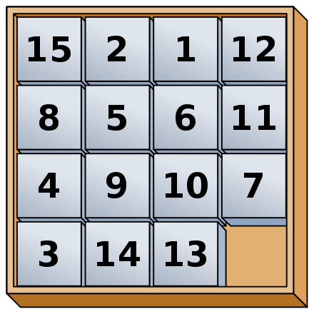
Two simple heuristics for the 15-puzzle are
Admissibility guarantees that the output solution is optimal. Here's a sketch of the proof:
Search stops when goal state becomes top option in frontier (not when goal is first discovered). Suppose we have found goal with path P and cost C. Consider a partial path X in the frontier. Its estimated cost must be \(\ge C\). Since our heuristic is admissible, the true cost of extending X to reach the goal must also be \( \ge C\). So extending X can't give us a better path than P.
There are many variants of A*, mostly hacks that may help for some problems and not others. See this set of pages for extensive implementation detail Amit Patel's notes on A*.
\(A^*\) decays gracefully if admissibility is relaxed. If the heuristic only slightly overestimates the distance, then the return path should be close to optimal. This is called "suboptimal" search. Non-admissible heuristics are particularly useful when there are many alternate paths of similar (or even the same) cost, as in a very open maze. The heuristic is adjusted slightly to create a small preference for certain of these similar paths, so that search focuses on extending the preferred paths all the way out to the goal. See Amit Patel's notes for details.
In some search problems, notably speech recognition, the frontier can get extremely large. "Beam search" algorithms prune states with high values of f, frequently restricting the queue to some fixed length N. Like suboptimal search, this sabotages guarantees of optimality. However, in practice, it may be extremely unlikely that these poorly-rated states can be extended to a good solution.
Another well-known variant is iterative deepening A*. Remember that iterative deepening is based on a version of DFS ("length-bounded") in which search is stopped when the path reaches a target length k. Iterative deepening A* is similar, but search stops if the A* estimated cost f(s) is larger than k.
Another optimization involves building a "pattern database." This is a database of partial problems, together with the cost to solve the partial problem. The true solution cost for a search state must be at least as high as the cost for any pattern it contains.
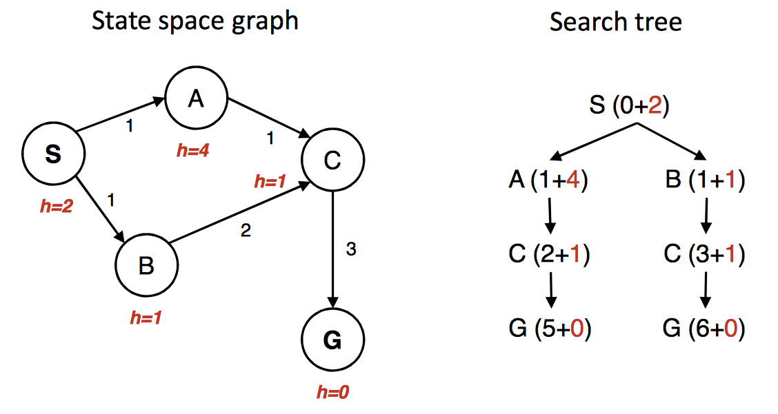
\(A^*\) finds the optimal path only when you do the bookkeeping correctly. The details are somewhat like UCS, but there are some new issues. Consider the following example (artificially cooked up for the purpoose of illustration).
(from Berkeley CS 188x materials)
The state graph is shown on the left, with the h value under each state. The right shows a quick picture of the search process. Walking through the search in more detail:
First we put S in the queue with estimated cost 2, i.e. g(S) = 0 plus h(S) = 2.
We remove S from the queue and add its neighbors. A has estimated cost 5 and B has estimated cost 2. S is now done/closed.
We remove B from the queue and add its neighbor C. C has estimated cost 4. B is now done/closed.
We remove C from the queue. One of its neighbors (A) is already in the queue. So we only need to add G. G has cost 6. C is now done/closed.
We remove A from the queue. Its neighbors are all done, so we have nothing to do. A is now done.
We remove G from the queue. It's the goal, so we halt, reporting that the best path is SBCG with cost 6.
Oops. The best path is through A and has actual cost 5. But heuristic was admissible. What went wrong? Obviously we didn't do our bookkeeping correctly.
The algorithm we inherited from from UCS only updates costs for nodes that are in the frontier. In this example, paths through B look better at the start. So SBCG reaches C and G first. C and G are marked done/closed. And then we see the shorter path SAC. Updating the cost of C won't help because it's in the done/closed set.
Fix: when we update the cost of a node in the closed/done set, put that node back into the frontier (priority queue).
The problem with shorter paths to old states is simplified if our heuristic is "consistent." That is, if we can get from s to s' with cost c(s,s'), we must have
\( h(s) \le c(s,s') + h(s') \)
So as we follow a path away from start state, our estimated cost f never decreases. Useful heuristics are often consistent. For example, the straight-line distance is consistent because of the triangle inequality.
When the heuristic is consistent, we never have to update the path length for a node that is in the done/closed set. (Though we may still have to update path lengths for nodes in the frontier.)
We can view UCS as A* with a heuristic function h that always returns zero. This heuristic is consistent, so updates to costs in UCS involve only states in the frontier.