
from Wikipedia
What do words mean?
Why do we care?
What are they useful for?
In Russell and Norvig style: what concepts does a rational agent use to do its reasoning?
We can use models of word meaning to model how humans process language. They can also speed up language processing tasks such as
Seen from a neural net perspective, the key issue is that one-hot representations of words don't scale well. E.g. if we have a 100,000 word vocabulary, we use vectors of length 100,000. We should be able to give each word a distinct representation using a lot fewer parameters.
Here is the definition of "bird" from Oxford Living Dictionaries (Oxford University Press)
"A warm-blooded egg-laying vertebrate animal distinguished by the possession of feathers, wings, a beak, and typically by being able to fly."
Back in the Day, people tried to turn such definitions into representations with the look and feel of formal logic:
isa(bird, animal)
AND has(bird, wings)
AND flies(bird)
AND if female(bird), then lays(bird,eggs) ....
The above example is not only incompete, but also has a bug: not all birds fly. It also contains very little information on what birds look like or how they act, so not much help for recognition. Recall from our early classifier lectures that people rely heavily on context to decide what name to give an object.
General problems with this style of meaning representation:
For each word, we'd like to learn
Many meanings can be expressed by a word that's more fancy or more plain. E.g. bellicose (fancy) and warlike (plain) mean the same thing. Words can also describe the same property in more or less complimentary terms, e.g. plump (nice) vs. fat (not nice). This leads to jokes about "irregular conjugations" such as
A more subtle problem with these logic-style representations of meaning is that people are are sensitive to the overall structure of the vocabulary. Although some words are seen as synonyms, it's more common that distinct words are seen as having distinct senses, even when the speaker cannot explain what is different about their meaning.
The "Principle of Contrast" states that differences in form imply differences in meaning. (Eve Clark 1987, though idea goes back earlier). For example, kids will say things like "that's not an animal, that's a dog." Adults have a better model that words can refer to more or less general categories of objects, but still make mistakes like "that's not a real number, it's an integer." Apparent synonyms seem to inspire a search for some small difference in meaning. For example, how is "graveyard" different from "cemetery"? Perhaps cemeteries are prettier, or not adjacent to a church, or fancier, or ...
People can also be convinced that two meanings are distinct because an expert says they are, even when they cannot explain how they differ (an observation originally due to the philosopher Hilary Putnam). For example, pewter (used to make food dishes) and nickel silver (used to make keys for instruments) are similar looking dull silver-colored metals used as replacements for silver. The difference in name tells people that they must be different. But most people would have to trust an expert because they can't tell them apart. Even fewer could tell you that they are alloys with these compositions:
A different approach to representing word meanings, which has recently been working better in practice is to observe how people use each word.
"You shall know a word by the company it keeps" (J. R. Firth, 1957)
People have a lot of information to work with, e.g. what's going on when the word was said, how other people react to it, even actual explanations from other people. Most computer algorithms only get to see running text. So we approximate this idea by observing which words occur in the same textual context. That is words that occur together often share elements of meaning.
We can also figure out an unfamiliar word from examples in context:
Authentic biltong is flavored with coriander.
John took biltong on his hike.
Antelope biltong is better than ostrich biltong .
The first context suggests that biltong is food. The second context suggests that it isn't perishable. The third suggests it involves meat.
This would probably be enough information for you to use the word biltong in a sentence, as if you completely understood what it meant. For some tasks, that might be enough. However, you might want to know a bit more detail before deciding whether to eat some. We've all heard stories of travellers who ordered some mystery dish off a foreign language menu and it turned out to be something they hated. An important unsolved problem is hold to "ground" meanings in the real world, i.e. relate the meaning of a world to observable properties such as appearance and taste.
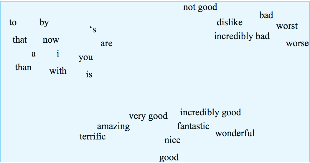
Idea: let's represent each word as a vector of numerical feature values.
These feature vectors are called word embeddings. In an ideal world, the embeddings might look like this embedding of words into 2D, except that the space has a lot more dimensions. (In practice, a lot of massaging would be required to get a picture this clean.) Our measures of similarity will be based on what words occur near one another in a text data corpus, because that's the type of data that's available in quantity.
from Jurafsky and Martin
Feature vectors are based on some context that the focus word occurs in. There are a continuum of possible contexts, which will give us different information:
Close neighbors tend to tell you about the word's syntactic properties (e.g. part of speech). Nearby words tend to tell you about its main meaning. Features from the whole document tend to tell you what topic area the word comes from (e.g. math letures vs. Harry Potter).
For example, we might count how often each word occurs in each of a group of documents, e.g. the following table of selected words that occur in various plays by Shakespeare. These counts give each word a vector of numbers, one per document.
| As You Like It | Twelfth Night | Julius Caesar | Henry V | |
|---|---|---|---|---|
| battle | 1 | 0 | 7 | 13 |
| good | 114 | 80 | 62 | 89 |
| food | 36 | 58 | 1 | 4 |
| wit | 20 | 15 | 2 | 3 |
We can also used these word-document matrices to produce a feature vector for each document, describing its topic. These vectors would typically be very long (e.g. one value for every word that is used in any of the documents). This representation is primarily used in document retrieval, which is historically the application for which many vector methods were developed.
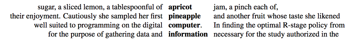
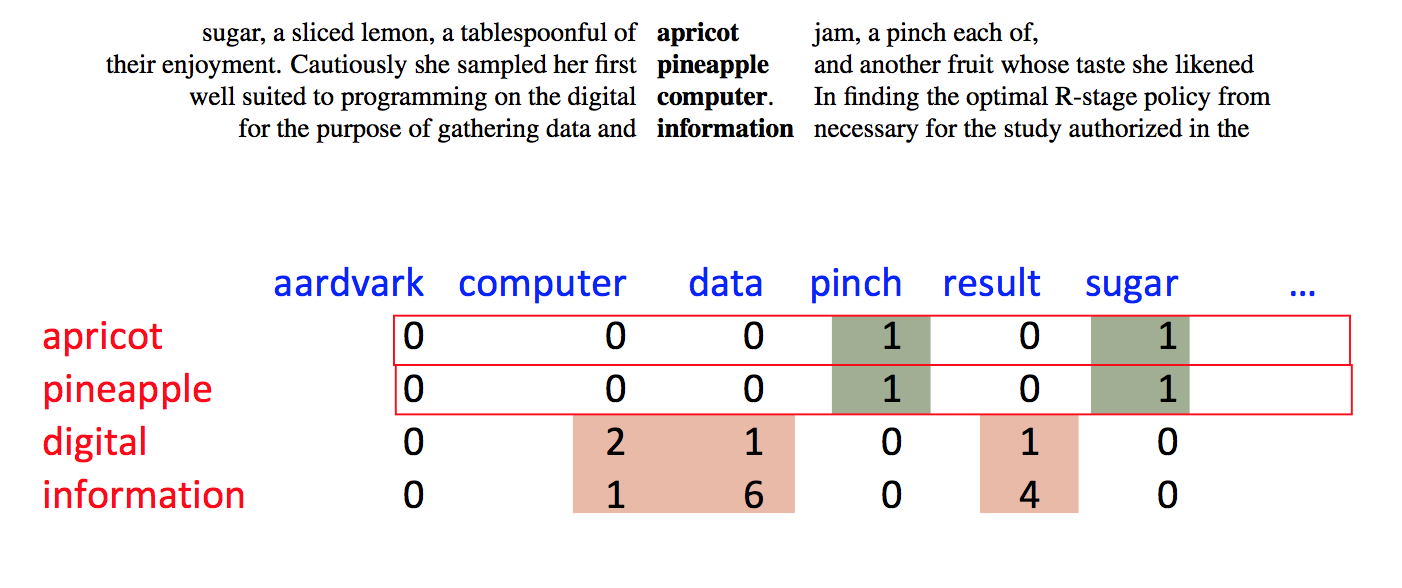
Alternative, we can use nearby words as context. So this example from Jurafsky and Martin shows sets of 7 context words to each side of the focus word.
Our 2D data table then relates each focus word (row) to each context word (column). So it might look like this, after processing a number of documents.
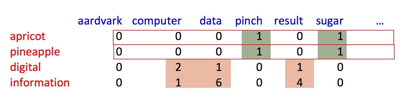
These raw count vectors will require some massaging to make them into nice feature representations. (We'll see the details later.) And they don't provide a complete model of word meanings. However, as we've seen earlier with neural nets, they provide representations that are good enough to work well in many practical tasks.
Suppose we have a vector of word counts for each document. How do we measure similarity between documents?
Notice that short documents have fewer words than longer ones. So we normally consider only the direction of these feature vectors, not their lengths. So we actually want to compare the directions of these vectors. The smaller the angle between them, the more similar they are.
(2, 1, 0, 4, ...)
(6, 3, 0, 8, ...) same as previous
(2, 3, 1, 2, ...) different
This analysis applies also to feature vectors for words: rare words have fewer observations than common ones. So, again, we'll measure similarity using the angle between feature vectors.
The actual angle is hard to work with, e.g. we can't compute it without calling an inverse trig function. It's much easier to approximate the angle with its cosine.
Recall what the cosine function looks like
What happens past 90 degrees? Oh, word counts can't be negative! So our vectors all live in the first quadrant, so their angles can't differ by more than 90 degrees.
Recall a handy formula for computing the cosine of the angle \(\theta\) between two vectors:
input vectors \(v = (v_1,v_2,\ldots,v_n) \) and \(w = (w_1,w_2,\ldots,w_n) \)
dot product: \( v\cdot w = v_1w_1 + ... + v_nw_n\)
\( \cos(\theta) = \frac{v \cdot w}{|v||w|} \)
So you'll see both "cosine" and "dot product" used to describe this measure of similarity.
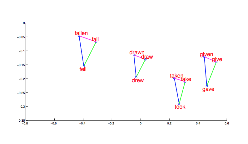
After significant cleanup (which we'll get to), we can produce embeddings of words in which proximity in embedding space mirrors similarity of meaning. For example, in the picture below (from word2vec), morphologically related words end up clustered. And, more interesting, the shape and position of the clusters are the same for different stems.
from Mikolov,
NIPS 2014
Notice that this picture is a projection of high-dimensional feature vectors onto two dimensions. And they authors are showing us only selected words. It's very difficult to judge the overall quality of the embeddings.
Word embedding models are evaluated in two ways:
Suppose we find a bunch of pairs of words illustrating a common relation, e.g. countries and their capitals in the figure below. The vectors relating the first word (country) to the second word (capital) all go roughly in the same direction.
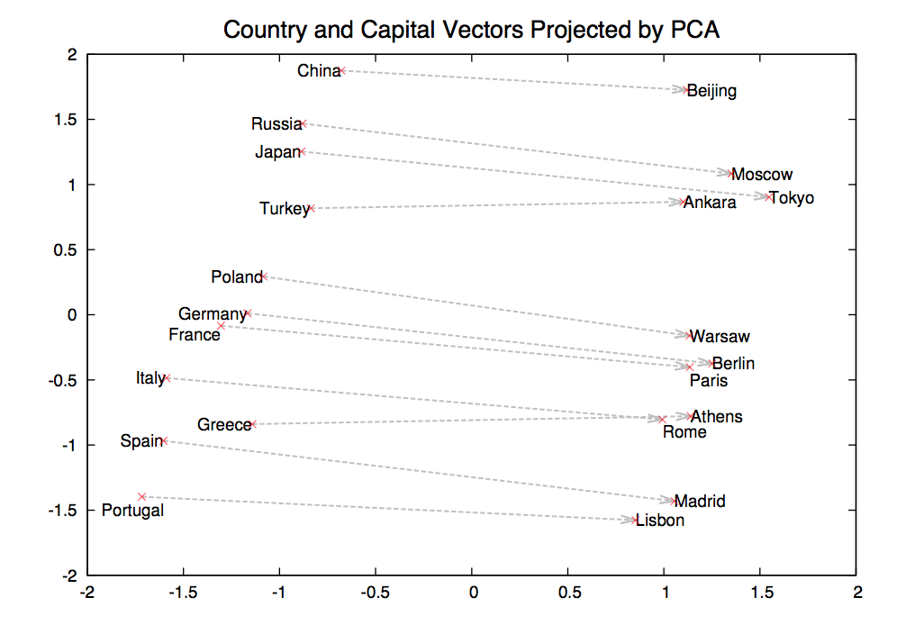
from Mikolov,
NIPS 2014
We can get the meaning of a short phrase by adding up the vectors for the words it contains. This gives us a simple version of "compositional semantics," i.e. deriving the meaning of a phrase from the meanings of the words in it. We can also do simple analogical reasoning by vector addition and subtraction. So if we add up
vector("Paris") - vector("France") + vector("Italy")
We should get the answer to the analogy question "Paris is to France as ?? is to Italy". The table below shows examples where this calculation produced an embedding vector close to the right answer:
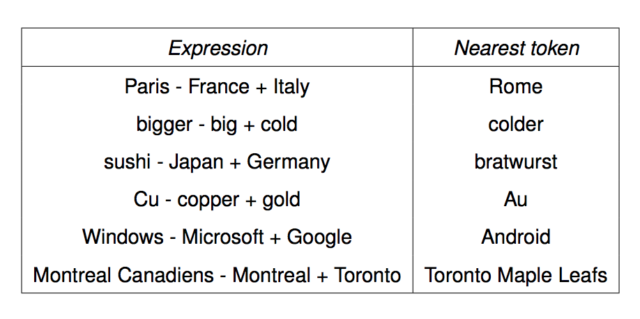
from Mikolov,
NIPS 2014
Here's one of our example tables of raw word counts (from Jurafsky and Martin)
| As You Like It | Twelfth Night | Julius Caesar | Henry V | |
|---|---|---|---|---|
| battle | 1 | 0 | 7 | 13 |
| good | 114 | 80 | 62 | 89 |
| food | 36 | 58 | 1 | 4 |
| wit | 20 | 15 | 2 | 3 |
Raw word count vectors don't work very well. Two basic problems need to be fixed:
We'll first see older methods in which these two steps are distinct. We'll then see word2vec, which accomplishes both via one procedure.
Why don't raw word counts work well?
In terms of the item we're trying to classify
As we saw above, this can be handled by using the direction (not the magnitude) of each count vector. When comparing two vectors, we look at the angle between them (or its cosine or a normalized dot product).
But there's also a related issue, which isn't fixed by comparing angles. Consider the context words, i.e. the words whose counts are entries in our vectors. Then
We need to normalize our individual counts to minimize the impact of these effects.
TF-IDF normalization maps word counts into a better measure of their importance for classification. It is a bit of a hack, but one that has proved very useful in document retrieval. To match the historical development, suppose we're trying to model the topic of a document based on counts of how often each word occurs in it.
Suppose that we are looking at a particular focus word in a particular focus document. The TF-IDF feature is the product of TF (normalized word count) and IDF (inverse document frequency).
Warning: neither TF nor IDF has a standard definition, and the most common definitions don't match what you might guess from the names. See Wikipedia Here is one of many variations on how to define them.
To keep things simple, let's assume that our word occurs at least once. It's pretty much universal that these normalization methods leave 0 counts unchanged.
To compute TF, we transform the raw count c for the word onto a log scale. That is, we replace it by \(\log{c}\). Across many different types of perceptual domains (e.g. word frequency, intensity of sound or light) studies of humans suggest that our perceptions are well modelled by a log scale. Also, the log transformation reduces the impact of correlations (repeated words) within a document.
However, \(\log{c}\) maps 1 to zero and exaggerates the importance of very rare words. So it's more typical to use
TF = \(\log_{10}(1+c)\)
The document frequency (DF) of the word, is df/N, where N is the total number of documents and df is the number of documents that our word appears in. When DF is small, our word provides a lot of information about the topic. When DF is large, our word is used in a lot of different contexts and so provides little information about the topic.
The normalizing factor IDF is also typically put through a log transformation, for the same reason that we did this to TF:
IDF = \( \log_{10}(N/df)\)
To avoid exaggerating the importance of very small values of N/df, it's typically better to use this:
IDF = \( \log_{10}(1+ N/df)\)
The final number that goes into our vector representation is TF \(\times\) IDF. That is, we multiply the two quantities even though we've already put them both onto a log scale. I did say this was a bit of a hack, didn't I?
Let's switch to our other example of feature vectors: modelling a word's meaning on the basis of words seen near it in running text. We still have the same kinds of normalization/smoothing issues.
Here's a different (but also long-standing) approach to normalization. We've picked a focus word w and a context word c. We'd like to know how closely our two words are connected. That is, do they occur together more often than one might expect for independent draws?
Suppose that w occurs with probability P(w) and c with probability P(c). If the two were appearing independently in the text, the probability of seeing them together would be P(w)P(c). Our actual observed probability is P(w,c). So we can use the following fraction to gauge how far away they are from independent:
\( \frac {P(w,c)}{P(w)P(c)} \)
Example: consider "of the" and "three-toed sloth." The former occurs a lot more often. However, that's mostly because its two constituent words are both very frequent. The PMI normalizes by the frequencies of the constituent words.
Putting this on a log scale gives us the pointwise mutual information (PMI)
\( I(w,c) = \log_2(\frac {P(w,c)}{P(w)P(c)}) \)
When one or both words are rare, there is high sampling error in their probabilities. E.g. if we've seen a word only once, we don't know if it occurs once in 10,000 words or once in 1 million words. So negative values of PMI are frequently not reliable. This observation leads some researchers to use the positive PMI (PPMI):
PPMI = max(0,PMI)
Warning: negative PMI values may be statistically significant, and informative in practice, if both words are quite common. For example, "the of" is infrequent because it violates English grammar. There have been some computational linguistics algorithms that exploit these significant zeroes. E.g. see Mohri and Roark 2005 "Structural Zeros vs. Sampling Zeros".
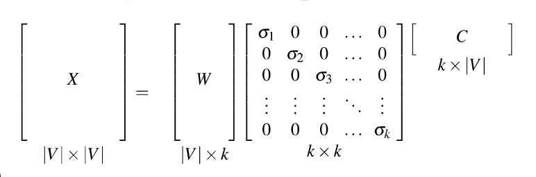
Both TF-IDF and PMI methods create vectors that contain informative numbers but still very long and sparse. For most applications, we would like to reduce these to short dense vectors that capture the most important dimensions of variation. A traditional method of doing this uses the singular value decomposition (SVD).
Theorem: any rectangular matrix can be decomposed into three matrices:
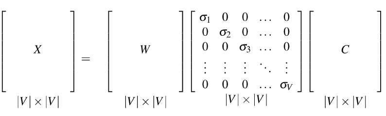
from Dan Jurafsky at Stanford.
In the new coordinate system (the input/output of the S matrix), the information in our original vectors is represented by a set of orthogonal vectors. The values in the S matrix tell you how important each basis vector is, for representing the data. We can make it so that weights in S are in decreasing order top to bottom.
It is well-known how to compute this decomposition. See a scientific computing text for methods to do it accurately and fast. Or, much better, get a standard statistics or numerical analysis package to do the work for you.
Recall that our goal was to create shorter vectors. The most important information lies in the top-left part of the S matrix, where the S values are high. So let's consider only the top k dimensions from our new coordinate system: The matrix W tells us how to map our input sparse feature vectors into these k-dimensional dense feature vectors.
 from Dan Jurafsky at Stanford.
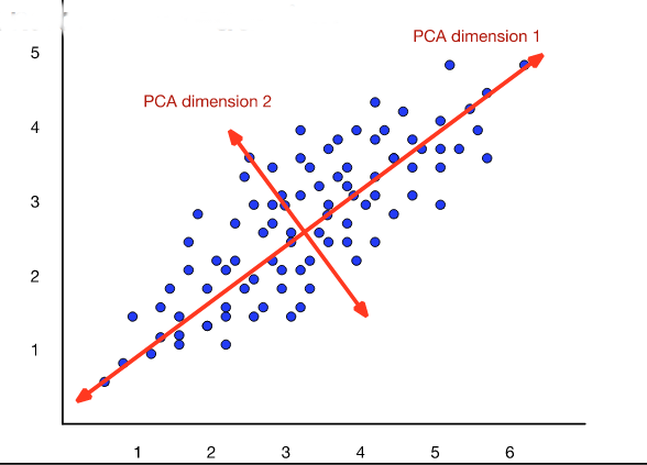
The new dimensions are called the "principal components." So this technique is often called a principal component analysis (PCA). When this approach is applied to analysis of document topics, it is often called "latent semantic analysis" (LSA).
 from Dan Jurafsky at Stanford.
Bottom line on SVD/PCA
The word2vec (aka skip-gram) algorithm is a newer algorithm that does normalization and dimensionality reduction in one step. That is, it learns how to embed words into an n-dimensional feature space. The algorithm was introduced in a couple papers by Tomas Mikolov et al in 2013. However, it's pretty much impossible to understand the algorithm from those papers, so the following derivation is from later papers by Yoav Goldberg and Omer Levy. Two similar embedding algorithms (which we won't cover) are the CBOW algorithm from word2vec and the GloVe algorithm from Stanford.
In broad outline word2vec has three steps
A pair (w,c) is considered "similar" if the dot product \(w\cdot c\) is large.
For example, our initial random embedding might put "elephant" near "matchbox" and far from "rhino." Our iterative adjustment would gradually move the embedding for "rhino" nearer to the embedding for "elephant."
Two obvious parameters to select. The dimension of the embedding space would depend on how detailed a representation the end user wants. The size of the context window would be tuned for good performance.
Problem: a great solution for the above optimization problem is to map all words to the same embedding vector. That defeats the purpose of having word embeddings.
Suppose we had negative examples (w,c'), in which c' is not a likely context word for w. Then we could make the optimization move w and c' away from each other. Revised problem: our data doesn't provide negative examples.
Solution: Train against random noise, i.e. randomly generate "bad" context words for each focus word.
The negative training data will be corrupted by containing some good examples, but this corruption should be a small percentage of the negative training data.
Another mathematical problem happens when we consider a word w with itself as context. The dot product \(w \cdot w\) ls large, by definition. But, for most words, w is not a common context for itself, e.g. "dog dog" is not very common compared to "dog." So setting up the optimization process in the obvious way causes the algorithm to want to move w away from itself, which it obviously cannot do.
To avoid this degeneracy, word2vec builds two embeddings of each word w, one for w seen as a focus word and one for w used as a context word. The two embeddings are closely connected, but not identical. The final representation for w will be a concatenation of the two embedding vectors.
Our classifier tries to predict yes/no from pairs (w,c), where "yes" means c is a good context word for w.
We'd like to make this into a probabilistic model. So we run dot product through a sigmoid to produce a "probability" that (w,c) is a good word-context pair. These numbers probably aren't the actual probabilities, but we're about to treat them as if they are. That is, we approximate
\( P(\text{good} | w,c) \approx \sigma(w\cdot c). \)
By the magic of exponentials (see below), this means that the probability that (w,c) is not a good word-context pair is
\( P(\text{bad} | w,c) \approx \sigma(-w\cdot c). \)
Now we switch to log probabilities, so we can use addition rather than multiplication. So we'll be looking at e.g.
\(\log( P(\text{good} | w,c)) \approx \log(\sigma(w\cdot c)) \)
Suppose that D is the positive training pairs and D' is the set of negative training pairs. So our iterative refinement algorithm adjusts the embeddings (both context and word) so as to maximize
\( \sum_{(w,c) \in D} \ \log(\sigma(w\cdot c)) + \sum_{(w,c) \in D'} \ \log(\sigma(-w\cdot c)) \)
That is, each time we read a new focus word w from the training data, we
Ok, so how did we get from \( P(\text{good} | w,c) = \sigma(w\cdot c) \) to \( P(\text{bad} | w,c) = \sigma(-w\cdot c) \)?
"Good" and "bad" are supposed to be opposites. So \( P(\text{bad} | w,c) = \sigma(-w\cdot c) \) should be equal to \(1 - P(\text{good}| w,c) = 1- \sigma(w\cdot c) \). I claim that \(1 - \sigma(w\cdot c) = \sigma(-w\cdot c) \).
This claim actually has nothing to do with the dot products. As a general thing \(1 - \sigma(x) = \sigma(-x) \). Here's the math.
Recall the definition of the sigmoid function: \( \sigma(x) = \frac{1}{1+e^{-x}} \).
\( \eqalign{ 1-\sigma(x) &=& 1 - \frac{1}{1+e^{-x}} = \frac{e^{-x}}{1+ e^{-x}} \ \ \text{ (add the fractions)} \\ &=& \frac{1}{1/e^{-x}+ 1} \ \ (\text{divide top and bottom by } e^{-x}) \\ &=& \frac{1}{e^x + 1} \ \ \text{(what does a negative exponent mean?)} \\ &=& \frac{1}{1 + e^x} = \sigma(-x)} \)
In order to get nice results from word2vec, the basic algorithm needs to be tweaked a bit to produce this good performance. Similar tweaks are frequently required by other similar algorithms.
In the basic algorithm, we consider the input (focus) words one by one. For each focus word, we extract all words within +/- k positions as positive context words. We also randomly generate a set of negative context words. This produces a set of positive pairs (w,c) and a set of negative pairs (w,c') that are used to update the embeddings of w, c, and c'.
Tweak 1: Word2vec uses more negative training pairs than positive pairs, by a factor of 2 up to 20 (depending on the amount of training data available).
You might think that the positive and negative pairs should be roughly balanced. However, that apparently doesn't work. One reason may be that the positive context words are definite indications of similarity, whereas the negative words are random choices that may be more neutral than actively negative.
Tweak 2: Positive training examples are weighted by 1/m, where m is the distance between the focus and context word. I.e. so adjacent context words are more important than words with a bit of separation.
The closer two words are, the more likely their relationship is strong. This is a common heuristic in similar algorithms.
For a fixed focus word w, negative context words are picked with a probability based on how often words occur in the training data. However, if we compute P(c) = count(c)/N (N is total words in data), rare words aren't picked often enough as context words. So instead we replace each raw count count(c) with \( (\text{count}(c))^\alpha\). The probabilities used for selecting negative training examples are computed from these smoothed counts.
\(\alpha\) is usually set to 0.75. But to see how this brings up the probabilities of rare words compared to the common ones, it's a bit easier if you look at \( \alpha = 0.5 \), i.e. we're computing the square root of the input. In the table below, you can see that large probabilities stay large, but very small ones are increased by quite a lot. After this transformation, you need to normalize the numbers so that the probabilities add up to one again.
x \(x^{0.75}\) \(\sqrt{x}\) .99 .992 .995 .9 .924 .949 .1 .178 .316 .01 .032 .1 .0001 .001 .01
This trick can also be used on PMI values (e.g. if using the methods from the previous lecture).
Ah, but apparently they are still unhappy with the treatment of very common and very rare words. So, when we first read the input training data, word2vec modifies it as follows:
This improves the balance between rare and common words. Also, deleting a word brings the other words closer together, which improves the effectiveness of our context windows.
The 2014 version of word2vec uses use 1 billion words to train embeddings for basic task.
For the word analogy tasks, they used an embedding with 1000 dimensions and about 33 billion words of training data. Performance on word analogies is about 66%.
By coomparison: children hear about 2-10 million words per year. Assuming the high end of that range of estimates, they've heard about 170 million words by the time they take the SAT. So the algorithm is performing well, but still seems to be underperforming given the amount of data it's consuming.
Word embeddings are a standard component of many systems for processing natural language. GloVe and ELMo are two competitors to word2vec. Recent work often extracts word embeddings from a language model, which can require even more data to train.
One popular recent language model, BERT large (Devlin 2018), is trained using a 24-layer network with 340M parameters with a training corpus of over 3G words. This kind of training requires specialized hardward clusters. Again, a direction for future research is to figure out why ok performance seems to require so much training data and compute power.
Original Mikolov et all papers:
Goldberg and Levy papers (easier and more explicit)