Two issues

Raw word count vectors don't work very well. Two basic problems need to be fixed:

• The raw counts require normalization.
• Word-count vectors are too long and sparse.

We'll first see older methods in which these two steps are distinct. We'll then see word2vec, which accomplishes both via one procedure.

Normalizing word counts

Why don't raw word counts work well?

In terms of the item we're trying to classify

• common words have larger feature values than rare words
• long documents have larger feature values than short ones

This problem is handled (as we saw in the last video) by using the direction (not the magnitude) of each count vector. When comparing two vectors, we look at the angle between them (or its cosine or a normalized dot product).

But there's also a related issue, which isn't fixed by comparing angles. Consider the context words, i.e. the words whose counts are entries in our vectors. Then

• Very frequent words (e.g. function words) don't tell you much about the meaning.
• Very rare words provide unreliable context, e.g. an uncommon word like "anteater" might appear in only certain documents about animals, in a random way.
• Local observations (e.g. within a document) are highly correlated, so importance isn't proportional to frequency.

We need to normalize our individual counts to minimize the impact of these effects.

TF-IDF

TF-IDF normalization maps word counts into a better measure of their importance for classification. It is a bit of a hack, but one that has proved very useful in document retrieval. To match the historical development, suppose we're trying to model the topic of a document based on counts of how often each word occurs in it.

Suppose that we are looking at a particular focus word in a particular focus document. The TF-IDF feature is the product of TF (normalized word count) and IDF (inverse document frequency).

Warning: neither TF nor IDF has a standard definition, and the most common definitions don't match what you might guess from the names. Here is one of many variations on how to define them.

To keep things simple, let's assume that our word occurs at least once. It's pretty much universal that these normalization methods leave 0 counts unchanged.

To compute TF, we transform the raw count c for the word onto a log scale. That is, we replace it by \(\log{c}\). Across many different types of perceptual domains (e.g. word frequency, intensity of sound or light) studies of humans suggest that our perceptions are well modelled by a log scale. Also, the log transformation reduces the impact of correlations (repeated words) within a document.

However, \(\log{c}\) maps 1 to zero and exaggerates the importance of very rare words. So it's more typical to use

TF = \(1+\log_{10}(c)\)

The document frequency (DF) of the word, is df/N, where N is the total number of documents and df is the number of documents that our word appears in. When DF is small, our word provides a lot of information about the topic. When DF is large, our word is used in a lot of different contexts and so provides little information about the topic.

The normalizing factor IDF is also typically put through a log transformation, for the same reason that we did this to TF:

IDF = \( \log_{10}(N/df)\)

To avoid exaggerating the importance of very small values of N/df, it's typically better to use this:

IDF = \( \log_{10}(1+ N/df)\)

The final number that goes into our vector representation is TF \(\times\) IDF. That is, we multiply the two quantities even though we've already put them both onto a log scale. I did say this was a bit of a hack, didn't I?

Pointwise mutual information (PMI)

Let's switch to our other example of feature vectors: modelling a word's meaning on the basis of words seen near it in running text. We still have the same kinds of normalization/smoothing issues.

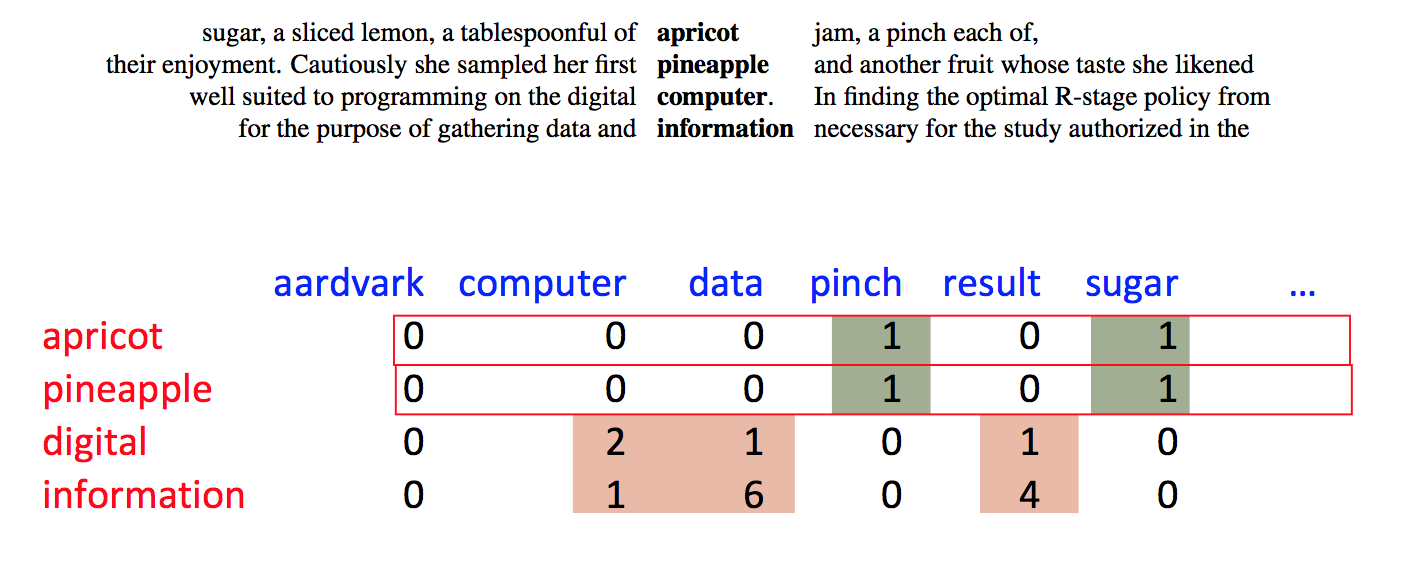
Here's a different (but also long-standing) approach to normalization. We've picked a focus word w and a context word c. We'd like to know how closely our two words are connected. That is, do they occur together more often than one might expect for independent draws?

Suppose that w occurs with probability P(w) and c with probability P(c). If the two were appearing independently in the text, the probability of seeing them together would be P(w)P(c). Our actual observed probability is P(w,c). So we can use the following fraction to gauge how far away they are from independent:

\( \frac {P(w,c)}{P(w)P(c)} \)

Example: consider "of the" and "three-toed sloth." The former occurs a lot more often. However, that's mostly because its two constituent words are both very frequent. The PMI normalizes by the frequencies of the constituent words.

Putting this on a log scale gives us the pointwise mutual information (PMI)

\( I(w,c) = \log_2(\frac {P(w,c)}{P(w)P(c)}) \)

When one or both words are rare, there is high sampling error in their probabilities. E.g. if we've seen a word only once, we don't know if it occurs once in 10,000 words or once in 1 million words. So negative values of PMI are frequently not reliable. This observation leads some researchers to use the positive PMI (PPMI):

PPMI = max(0,PMI)

Warning: negative PMI values may be statistically significant, and informative in practice, if both words are quite common. For example, "the of" is infrequent because it violates English grammar. There have been some computational linguistics algorithms that exploit these significant zeroes.

Singular value decomposition (SVD)

Both TF-IDF and PMI methods create vectors that contain informative numbers but still very long and sparse. For most applications, we would like to reduce these to short dense vectors that capture the most important dimensions of variation. A traditional method of doing this uses the singular value decomposition (SVD).

Theorem: any rectangular matrix can be decomposed into three matrices:

• W: maps original coordinates into new ones
• S: diagonal matrix of "singular values"
• C: maps new coordinates back to original ones

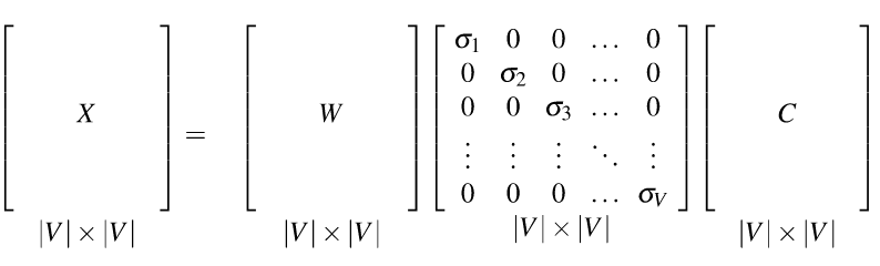
from Dan Jurafsky at Stanford.

In the new coordinate system (the input/output of the S matrix), the information in our original vectors is represented by a set of orthogonal vectors. The values in the S matrix tell you how important each basis vector is, for representing the data. We can make it so that weights in S are in decreasing order top to bottom.

It is well-known how to compute this decomposition. See a scientific computing text for methods to do it accurately and fast. Or, much better, get a standard statistics or numerical analysis package to do the work for you.

Recall that our goal was to create shorter vectors. The most important information lies in the top-left part of the S matrix, where the S values are high. So let's consider only the top k dimensions from our new coordinate system: The matrix W tells us how to map our input sparse feature vectors into these k-dimensional dense feature vectors.

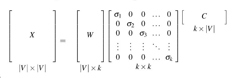from Dan Jurafsky at Stanford.

The new dimensions are called the "principal components." So this technique is often called a principal component analysis (PCA). When this approach is applied to analysis of document topics, it is often called "latent semantic analysis" (LSA).

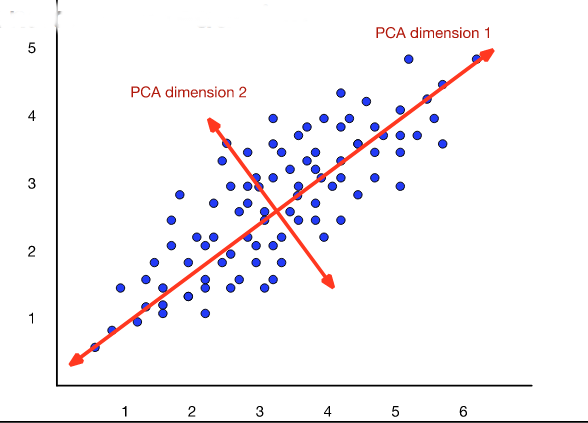from Dan Jurafsky at Stanford.

Bottom line on SVD/PCA

• Been around for ages. Lots of packages to do it for you.
• Helps human analysts figure out the important dimensions of variation.
• Works pretty well. Only the best newer methods do better.