Idea: let's represent each word as a vector of numerical feature values.
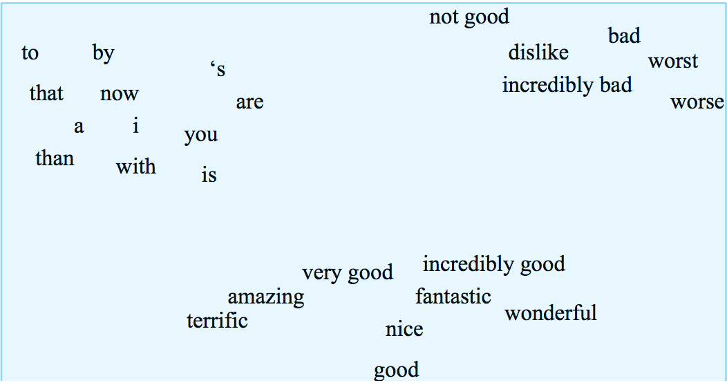
These feature vectors are called word embeddings. In an ideal world, the embeddings might look like this embedding of words into 2D, except that the space has a lot more dimensions. (In practice, a lot of massaging would be required to get a picture this clean.) Our measures of similarity will be based on what words occur near one another in a text data corpus, because that's the type of data that's available in quantity.

from Jurafsky and Martin
Feature vectors are based on some context that the focus word occurs in. There are a continuum of possible contexts, which will give us different information:
Close neighbors tend to tell you about the word's syntactic properties (e.g. part of speech). Nearby words tend to tell you about its main meaning. Features from the whole document tend to tell you what topic area the word comes from (e.g. math letures vs. Harry Potter).
For example, we might count how often each word occurs in each of a group of documents, e.g. the following table of selected words that occur in various plays by Shakespeare. These counts give each word a vector of numbers, one per document.
| As You Like It | Twelfth Night | Julius Caesar | Henry V | |
|---|---|---|---|---|
| battle | 1 | 0 | 7 | 13 |
| good | 114 | 80 | 62 | 89 |
| food | 36 | 58 | 1 | 4 |
| wit | 20 | 15 | 2 | 3 |
We can also used these word-document matrices to produce a feature vector for each document, describing its topic. These vectors would typically be very long (e.g. one value for every word that is used in any of the documents). This representation is primarily used in document retrieval, which is historically the application for which many vector methods were developed.
Alternative, we can use nearby words as context. So this example from Jurafsky and Martin shows sets of 7 context words to each side of the focus word.

Our 2D data table then relates each focus word (row) to each context word (column). So it might look like this, after processing a number of documents.

These raw count vectors will require some massaging to make them into nice feature representations. (We'll see the details later.) And they don't provide a complete model of word meanings. However, as we've seen earlier with neural nets, they provide representations that are good enough to work well in many practical tasks.
Suppose we have a vector of word counts for each document. How do we measure similarity between documents?
Notice that short documents have fewer words than longer ones. So we normally consider only the direction of these feature vectors, not their lengths. So we actually want to compare the directions of these vectors. The smaller the angle between them, the more similar they are.
(2, 1, 0, 4, ...)
(6, 3, 0, 8, ...) same as previous
(2, 3, 1, 2, ...) different
This analysis applies also to feature vectors for words: rare words have fewer observations than common ones. So, again, we'll measure similarity using the angle between feature vectors.
The actual angle is hard to work with, e.g. we can't compute it without calling an inverse trig function. It's much easier to approximate the angle with its cosine.
Recall what the cosine function looks like
What happens past 90 degrees? Oh, word counts can't be negative! So our vectors all live in the first quadrant, so their angles can't differ by more than 90 degrees.
Recall a handy formula for computing the cosine of the angle \(\theta\) between two vectors:
input vectors \(v = (v_1,v_2,\ldots,v_n) \) and \(w = (w_1,w_2,\ldots,w_n) \)
dot product: \( v\cdot w = v_1w_1 + ... + v_nw_n\)
\( \cos(\theta) = \frac{v \cdot w}{|v||w|} \)
So you'll see both "cosine" and "dot product" used to describe this measure of similarity.
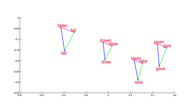
After significant cleanup (which we'll get to), we can produce embeddings of words in which proximity in embedding space mirrors similarity of meaning. For example, in the picture below (from word2vec), morphologically related words end up clustered. And, more interesting, the shape and position of the clusters are the same for different stems.

from Mikolov,
NIPS 2014
Notice that this picture is a projection of high-dimensional feature vectors onto two dimensions. And they authors are showing us only selected words. It's very difficult to judge the overall quality of the embeddings.
Word embedding models are evaluated in two ways:
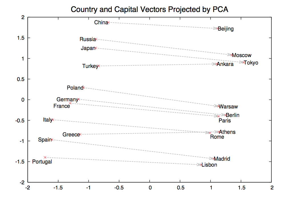
Suppose we find a bunch of pairs of words illustrating a common relation, e.g. countries and their capitals in the figure below. The vectors relating the first word (country) to the second word (capital) all go roughly in the same direction.

from Mikolov,
NIPS 2014
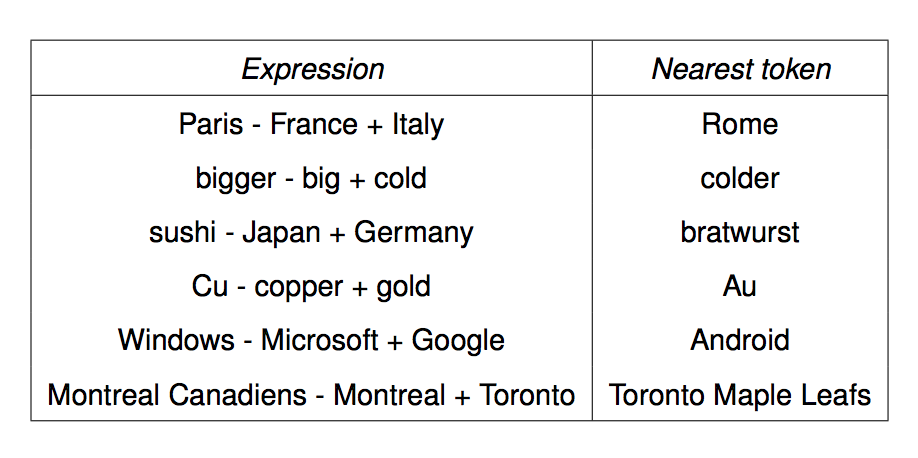
We can get the meaning of a short phrase by adding up the vectors for the words it contains. This gives us a simple version of "compositional semantics," i.e. deriving the meaning of a phrase from the meanings of the words in it. We can also do simple analogical reasoning by vector addition and subtraction. So if we add up
vector("Paris") - vector("France") + vector("Italy")
We should get the answer to the analogy question "Paris is to France as ?? is to Italy". The table below shows examples where this calculation produced an embedding vector close to the right answer:

from Mikolov,
NIPS 2014