Since this class depends on data structures, which has discrete math as a prerequisite, most people have probably seen some version of BFS, DFS, and state graphs before. If this isn't true for you, this lecture probably went too fast. Aside from the textbook, you may wish to browse web pages for CS 173, CS 225, and/or web tutorials on BFS/DFS.
Key parts of a state graph:
Task: find a low-cost path from start state to a goal state.
Some applications want a minimum-cost path. Others may be ok with a path whose cost isn't stupidly bad (e.g. no loops).
We can take a real-world map (below left) and turn it into a graph (below right). Notice that the graph is not even close to being a tree. So search algorithms have to actively prevent looping, e.g. by remember which locations they've already visited.
Mapping this onto a state graph:
On the graph, it's easy to see that there are many paths from
Northampton to Amherst, e.g. 8 miles via Hadley,
31 miles via Williamsburg and Whately.
Left below is an ASCII maze of the sort used in 1980's computer games.
R is the robot, G is the goal, F is a food pellet to collect
on the way to the goal. We no longer play games of this style,
but you can still find search problems with this kind of simple
structure. On the right is one path to the goal. Notice that
it has to double back on itself in two places.
Modelling this as a state graph:
Some mazes impose tight constraints on where the robot can go,
e.g. the bottom corridor in the above maze is only one cell wide.
Mazes with large open areas can have vast numbers of possible
solutions. For example, the maze below has many paths from start to
goal. In this case, the robot needs to move 10 steps right and 10
steps down. Since there are no walls constraining the order of right
vs. downward moves, there are \(20 \choose 10 \) paths of shortest
length (20 steps), which is about 185,000 paths.
We need to quickly choose one of these paths rather than wasting
time exploring all of them individually.
Game mazes also illustrate another feature that appears in some AI
problems: the AI gains access to the state graph as it explores.
E.g. at the start of the game, the map may actually look like this:
States may also be descriptins of the real world in terms of feature values.
For example, consider the
Missionaries and Cannibals puzzle. In the starting state, there
are three missionaries, three cannibals, and a boat on the left side of a
river. We need to move all six people to the right side, subject to
the following constraints:
The state of the world can be described by three variables: how many missionaries on
the left bank, how many cannibals on the left bank, and which bank the boat is on.
The state space is shown below:
In this example
In speech recognition, we need to transcribe an acoustic waveform into
to produce written text. We'll see details of this process later in the
course. For now, just notice that this proceeds word-by-word.
So we have a set of candidate transcriptions for the first part of
the waveform and wish to extend those by one more word. For example,
one candidate transcription might start with "The book was very" and
the acoustic matcher says that the next word sounds like "short" or "sort."
In this example
Speech recognition systems have vast state spaces. A recognition
dictionary may know about 100,000 different words. Because acoustic
matching is still somewhat error-prone, there may be many words that
seem to match the next section of the input. So the
currently-relevant states are constructed on demand, as we search.
Chess is another example of an AI problem with a vast state space.
For all but the simplest AI problems, it's easy for a search algorithm to
get lost.
The first two of these can send the program into an infinite loop. The
third and fourth can cause it to get lost, exploring states
very far from a reasonable path from the start to the goal.
Mazes
Puzzle
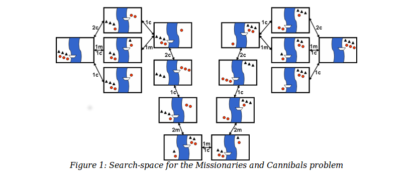 (from
Gerhard Wickler, U. Edinburgh)
(from
Gerhard Wickler, U. Edinburgh)
Speech recognition
Some high-level points