Gridworld pictures are from the U.C. Berkeley CS 188 materials (Pieter Abbeel and Dan Klein) except where noted.
Recall that we have a Markov Decision Process defined by
Recall that we are trying to maximize this sum. And we haven't actually defined the utility function U. But it should depends on the reward function R and give less weight to more distant rewards.
\(\sum_\text{sequences of states}\) P(sequence)U(sequence)
Suppose our actions were deterministic, then we could express the utility of each state in terms of the utilities of adjacent states like this:
\(U(s) = R(s) + \max_{a \in A} U(move(a,s)) \)
where move(a,s) is the state that results if we perform action a in state s. We are assuming that the agent always picks the best move (optimal policy).
Since our action does not, in fact, entirely control the next state s', we need to compute a sum that's weighted by the probability of each next state. The expected utility of the next state would be \(\sum_{s'\in S} P(s' | s,a)U(s') \), so this would give us a recursive equation
\(U(s) = R(s) + \max_{a \in A} \sum_{s'\in S} P(s' | s,a)U(s') \)
The actual equation should also include a reward delay multiplier \(\gamma\). Downweighting the contribution of neighboring states by \(\gamma\) causes their rewards to be considered less important than the immediate reward R(s). It also causes the system of equations to converge. So the final "Bellman equation" looks like this:
\(U(s) = R(s) + \gamma \max_{a \in A} \sum_{s'\in S} P(s' | s,a)U(s') \)
Specifically, this is the Bellman equation for the optimal policy.
Short version of why it converges. Since our MDP is finite, our rewards all have absolute value \( \le \) some bound M. If we repeatedly apply the Bellman equation to write out the utility of an extended sequence of actions, the kth action in the sequence will have a discounted reward \( \le \gamma^k M\). So the sum is a geometric series and thus converges if \( 0 \le \gamma < 1 \).
There's a variety of ways to solve MDP's and closely-related reinforcement learning problems:
The simplest solution method is value iteration. This method repeatedly applies the Bellman equation to update utility values for each state. Suppose \(U_k(s)\) is the utility value for state s in iteration k. Then
- initialize \(U_1(s) = 0 \), for all states s
- loop for k = 1 until the values converge
- \(U_{k+1}(s) = R(s) + \gamma \max_{a \in A} \sum_{s'\in S} P(s' | s,a)U_k(s') \)
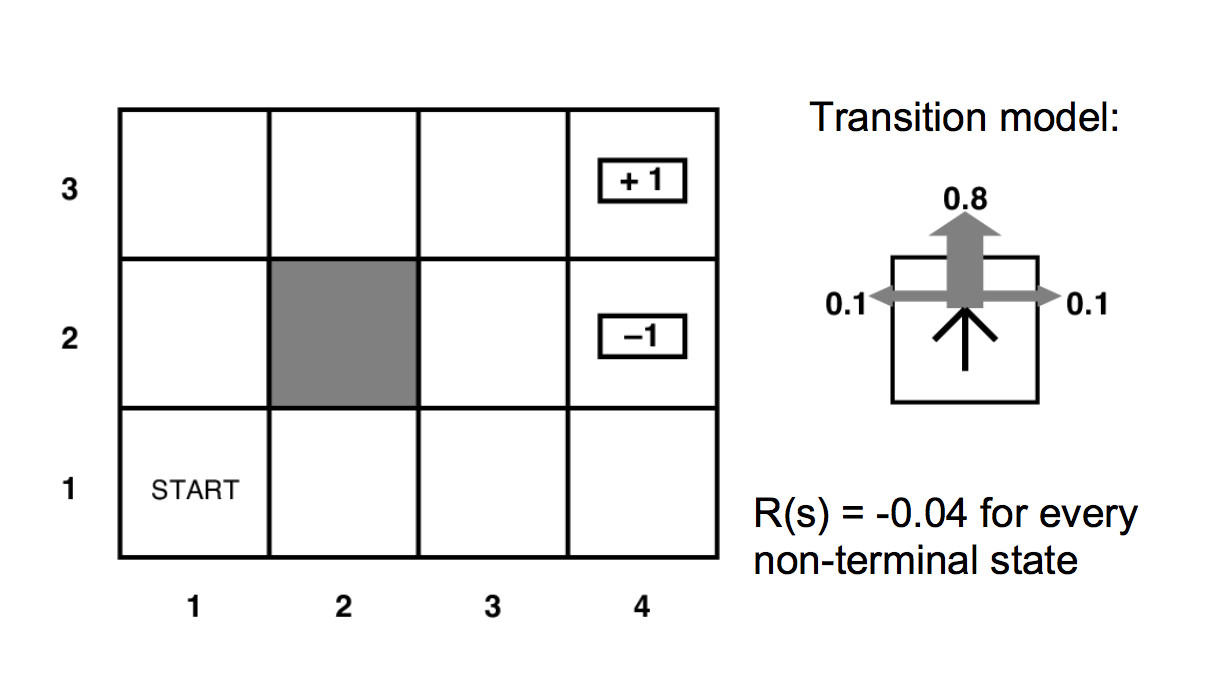
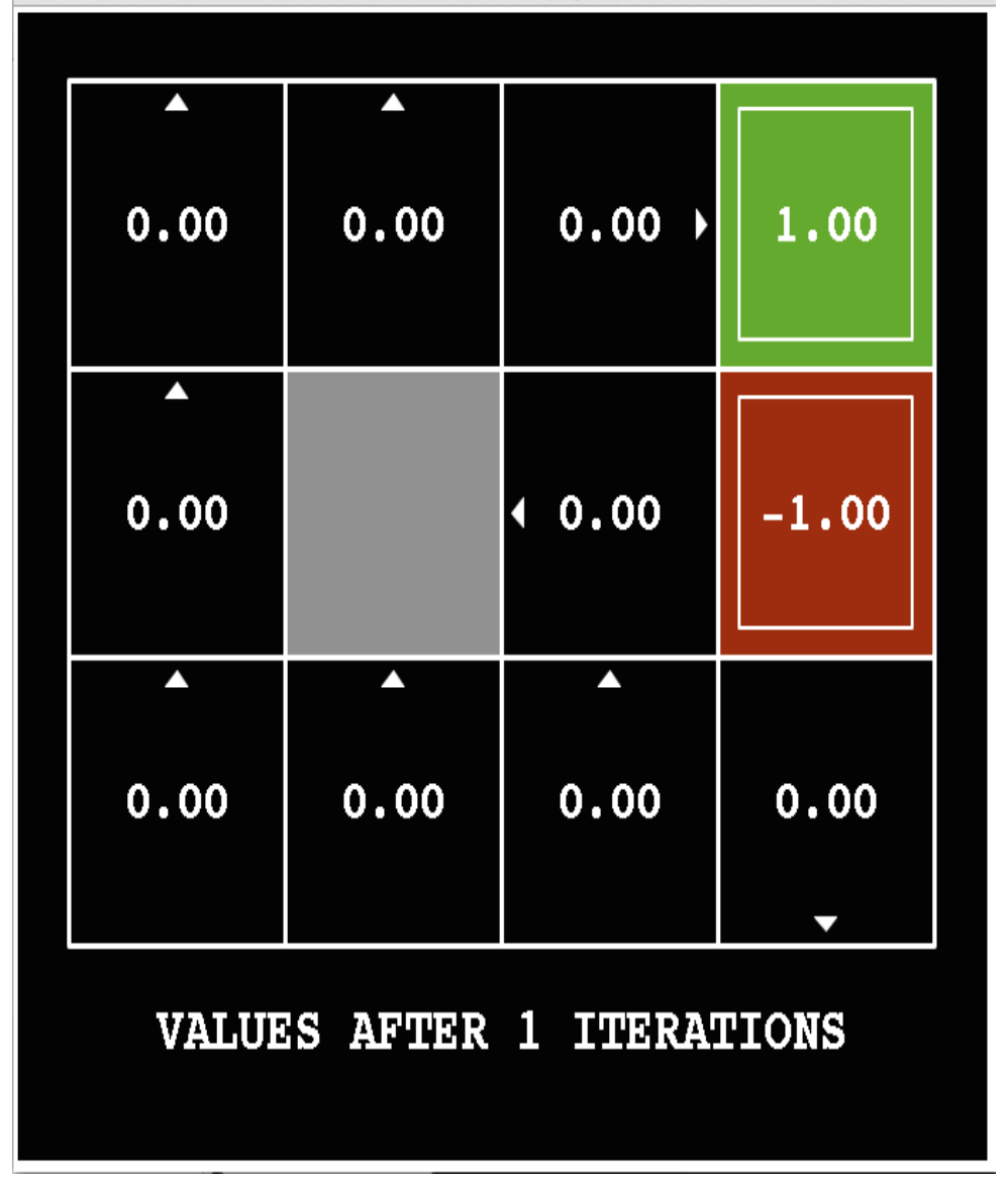
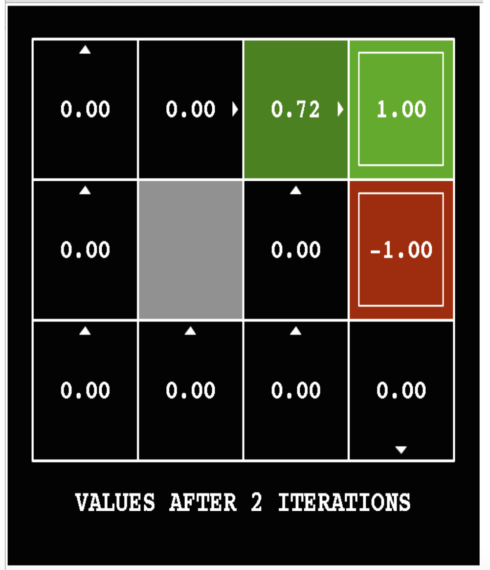
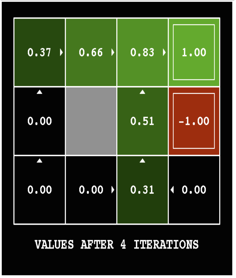
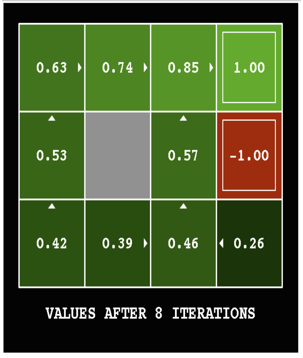
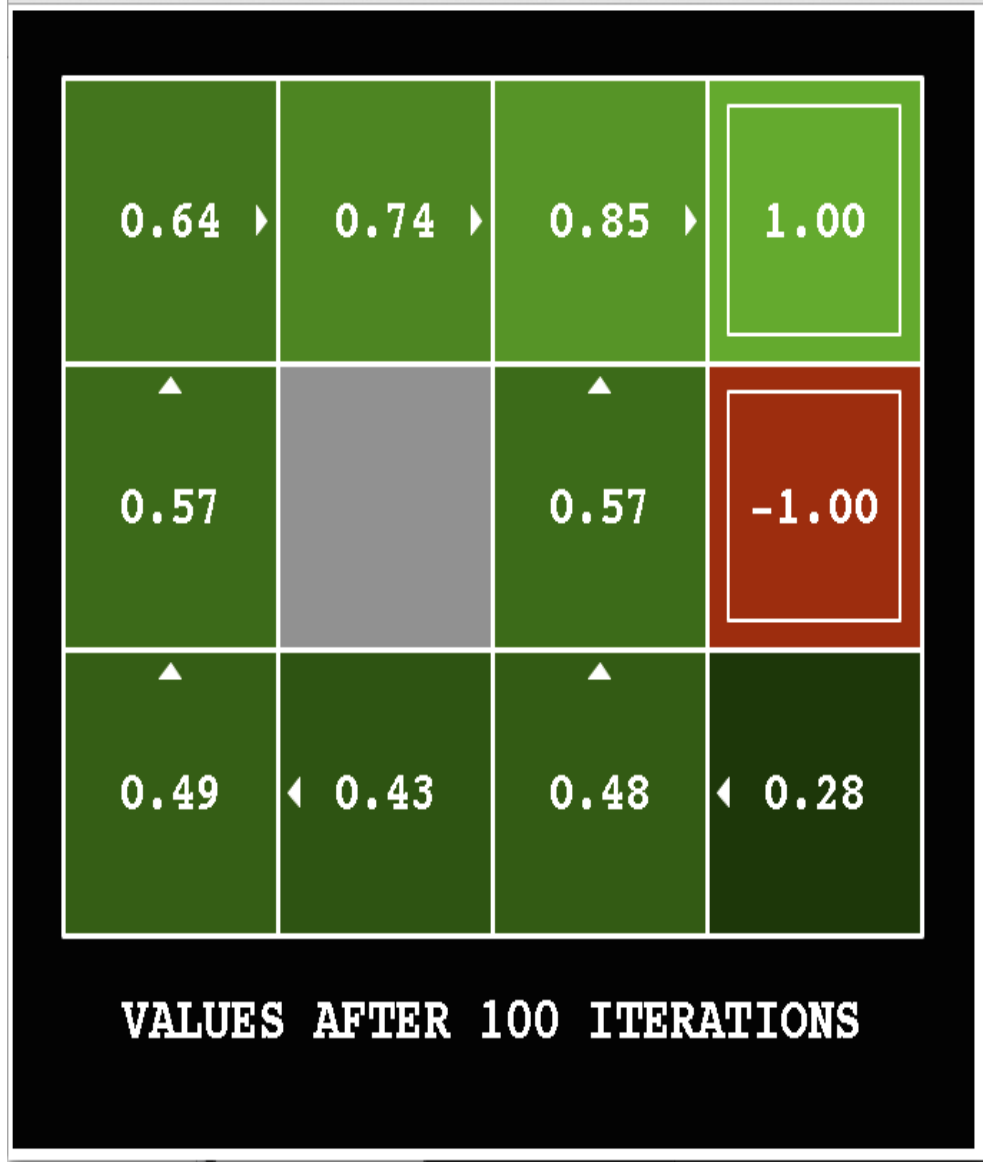
The following pictures show how the utility values change as the iteration progresses. The discount factor \(\gamma\) is set to 0.9 and the background reward is set to 0.
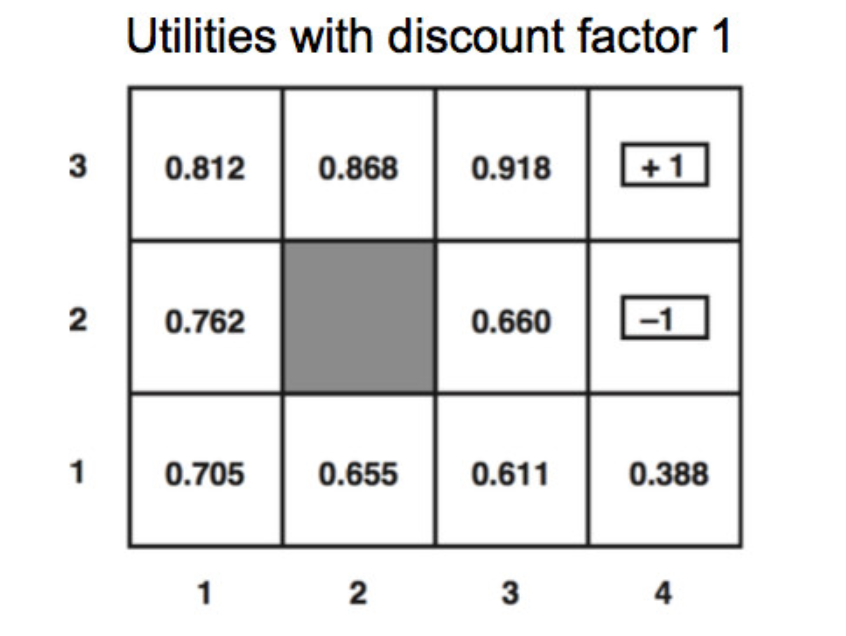
Here's the final output utilities for a variant of the same problem (discount factor \(\gamma = 1\) and the background reward is -0.04).
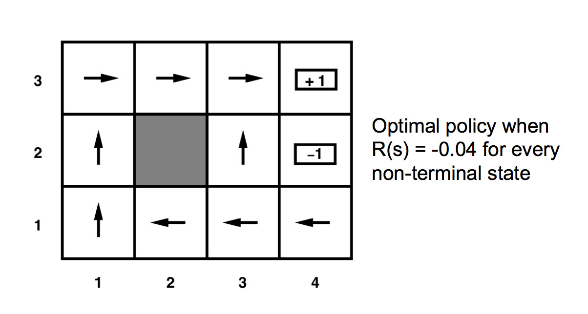
We can read a policy off the final utility values. We can't simply move towards the neighbor with the highest utility, because our agent doesn't always move in the direction we commanded. So the optimal policy requires examining a probabilitic sum:
\( \pi(s) = \text{argmax}_a \sum_{s'} P(s' | s,a) U(s') \)
You can play with a larger example in Andrej Karpathy's gridworld demo.
Some authors (notably the Berkeley course) use variants of the Bellman equation like this:
\( V(s) = \max_a \sum_{s'} P(s' | s,a) [R(s,a,s') + \gamma V(s')]\)
There is no deep change involved here. This is partly just pushing around the algebra. Also, passing more arguments to the reward function R allows a more complicated theory of rewards, i.e. depending not only on the new state but also the previous state and the action you used. If we use our simpler model of rewards, then this V(s) these can be related to our U(s) as follows
U(s) = R(s) + V(s)