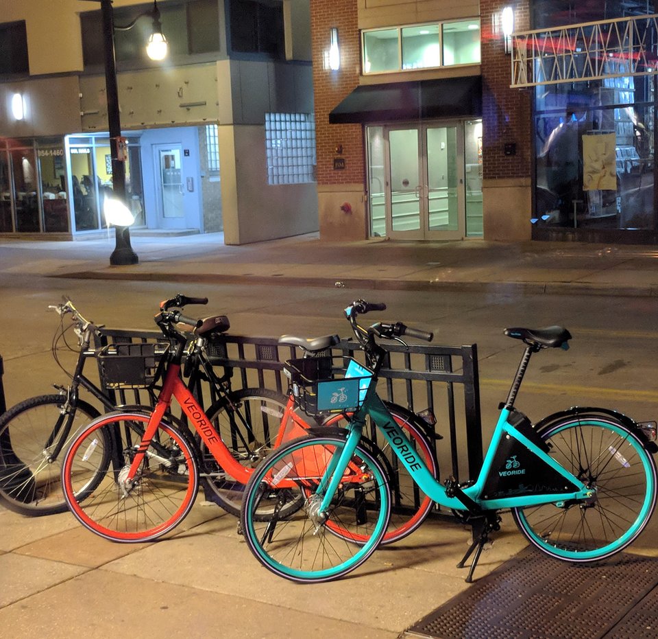
 Red and teal veoride bikes from
/u/civicsquid reddit post
Red and teal veoride bikes from
/u/civicsquid reddit post
       P(cause | evidence) =  P(evidence | cause) *  P(cause) / P(evidence)

       posterior            likelihood             prior     normalization
Example: We have two underlying types of bikes: veoride and standard. We observe a teal bike. What type should we guess that it is?
"Maximum a posteriori" (MAP) estimate chooses the type with the highest posterior probability:
pick the type X such that P(X | evidence) is highest
Suppose that type X comes from a set of types T. Then MAP chooses
\(\arg\!\max_{X \in T} P(X | \text{evidence}) \)
The argmax operator iterates through a series of values for the dummy variable (X in this case). When it determines the maximum value for the quantity (P(X | evidence) in this example), it returns the value for X that produced that maximum value.
Completing our example, we compute two posterior probabilities:
P(veoride | teal) = 0.905
P(standard | teal) = 0.095
The first probability is bigger, so we guess that it's a veoride. Notice that these two numbers add up to 1, as probabilities should.
P(evidence) can usually be factored out of these equations, because we are only trying to determine the relative probabilities. For the MAP estimate, in fact, we are only trying to find the largest probability. In our equation
P(cause | evidence) = P(evidence | cause) * P(cause) / P(evidence)
P(evidence) is the same for all the causes we are considering. Said another way, P(evidence) is the probability that we would see this evidence if we did a lot of observations. But our current situation is that we've actually seen this particular evidence and we don't really care if we're analyzing a common or unusual situation.
So Bayesian estimation often works with the equation
P(cause | evidence) \( \propto \) P(evidence | cause) * P(cause)
where we know (but may not always say) that the normalizing constant is the same across various such quantities.
Specifically, for our example
P(veoride | teal) = P(teal | veoride) * P(veoride) / P(teal)
P(standard | teal) = P(teal | standard) * P(standard) / P(teal)
P(teal) is the same in both quantities. So we can remove it, giving us
P(veoride | teal) \( \propto \) P(teal | veoride) * P(veoride) = 0.95 * 0.2 = 0.19
P(standard | teal) \( \propto \) P(teal | standard) * P(standard) = 0.025 * 0.8 = 0.02
So veoride is the MAP choice, and we never needed to know P(teal). Notice that the two numbers (0.19 and 0.02) don't add up to 1. So they aren't probabilities, even though their ratio is the ratio of the probabilities we're interested in.
As we saw above, our joint probabilities depend on the relative frequencies of the two underlying causes/types. Our MAP estimate reflects this by including the prior probability.
If we know that all causes are equally likely, we can set all P(cause) to the same value for all causes. In that case, we have
P(cause | evidence) \( \propto \) P(evidence | cause)
So we can pick the cause that maximizes P(evidence | cause). This is called the "Maximum Likelihood Estimate" (MLE).
The MLE estimate can be very inaccurate if the prior probabilities of different causes are very different. On the other hand, it can be a sensible choice if we have poor information about the prior probabilities.