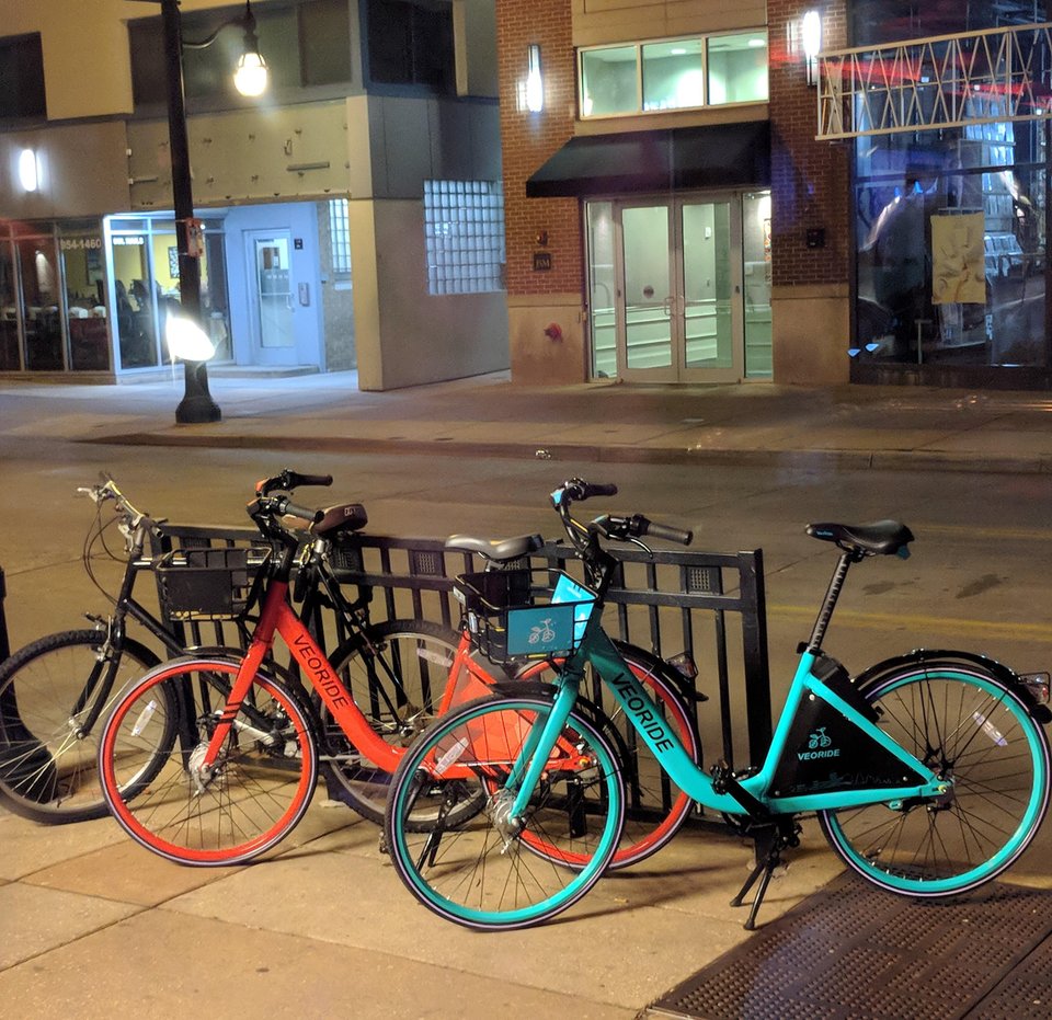
Red and teal veoride bikes from /u/civicsquid reddit post

Example: campus bikes

We have two types of bike (veoride and standard). Veorides are mostly teal (with a few exceptions), but other (privately owned) bikes rarely are.

Joint distribution for these two variables

                 veoride        standard     |
    teal            0.19          0.02       |   0.21
    red             0.01          0.78       |   0.79
                 ----------------------------
                    0.20          0.80

For this toy example, we can fill out the joint distribution table. However, when we have more variables (typical of AI problems), this isn't practical. The joint distribution contains

• too many probability values to estimate (\(2^n\) values for n variables)
• too many probability values to store

Bayes Rule

Remember that P(A | C) is the probability of A in a context where C is true. For example, the probability of a bike being teal increases dramatically if we happen to know that it's a veobike.

P(teal) = 0.21
P(teal | veoride) = 0.95 (19/20)

The formal definition:of conditional probability is

P(A | C) = P(A,C)/P(C)

Let's write this in the equivalent form P(A,C) = P(C) * P(A | C).

Flipping the roles of A and C (seems like middle school but just keep reading):

equivalently P(C,A) = P(A) * P(C | A)

P(A,C) and P(C,A) are the same quantity. (AND is commutative.) So we have

P(A) * P(C | A) = P(A,C) = P(C) * P(A | C)

So

P(A) * P(C | A) = P(C) * P(A | C)

So we have Bayes rule

P(C | A) = P(A | C) * P(C) / P(A)

Here's how to think about the pieces of this formula

       P(cause | evidence) =  P(evidence | cause) *  P(cause) / P(evidence)
         posterior            likelihood             prior     normalization

The normalization doesn't have a proper name because we'll typically organize our computation so as to eliminate it. Or, sometimes, we won't be able to measure it directly, so the number will be set at whatever is required to make all the probability values add up to 1.

Example: we see a teal bike. What is the chance that it's a veoride? We know

P(teal | veoride) = 0.95 [likelihood]
P(veoride) = 0.20 [prior]
P(teal) = 0.21 [normalization]

So we can calculate

P(veoride | teal) = 0.95 x 0.2 / 0.21 = 0.19/0.21 = 0.905

Why will this be useful?

In non-toy examples, it will be easier to get estimates for P(evidence | cause) than direct estimates for P(cause | evidence).

P(evidence | cause) tends to be stable, because it is due to some underlying mechanism. In this example, veoride likes teal and regular bike owners don't. In a disease scenario, we might be looking at the tendency of measles to cause spots, which is due to a property of the virus that is fairly stable over time.

P(cause | evidence) is less stable, because it depends on the set of possible causes and how common they are right now.

For example, suppose that a critical brake problem is discovered and Veoride suddenly has to pull bikes into the shop for repairs. So then only 2% of the bikes are veorides. Then we might have the following joint distribution. Now a teal bike is more likely to be standard rather than veoride.

                 veoride        standard     |
    teal            0.019          0.025     |   0.044
    red             0.001          0.955     |   0.956
                 ----------------------------
                    0.02           0.98

Dividing P(cause | evidence) into P(evidence | cause) and P(cause) allows us to easily adjust for changes in P(cause).