Joint probabilities

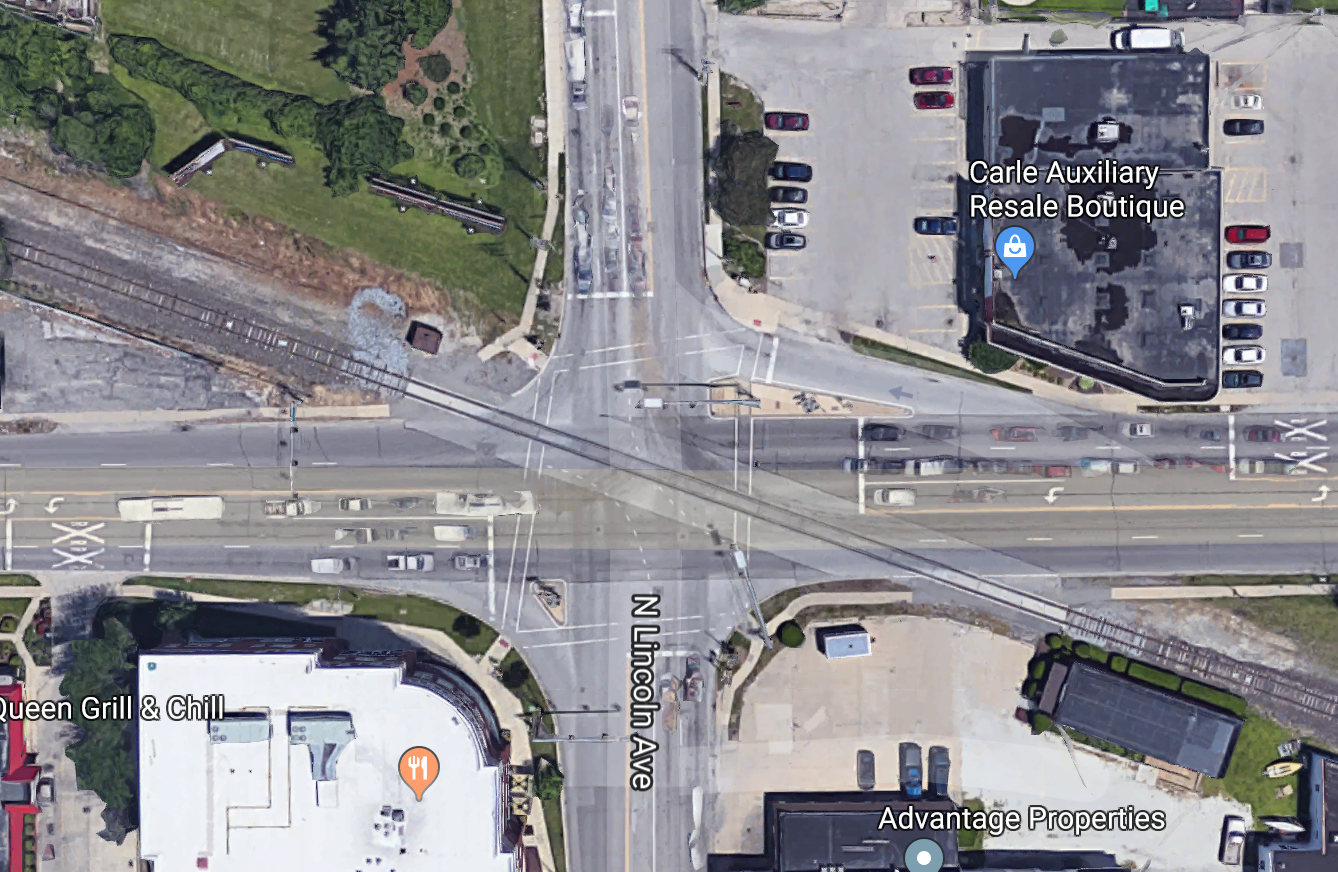
Here's a model of two variables for the University/Goodwin intersection:

                             E/W light                
                        green       yellow   red
 N/S light   green        0          0       0.2      
             yellow       0          0       0.1      
             red         0.5         0.1     0.1

To be a probability distribution, the numbers must add up to 1 (which they do in this example).

Most model-builders assume that probabilities aren't actually zero. That is, unobserved events do occur but they just happen so infrequently that we haven't yet observed one. So a more realistic model might be

                             E/W light              
                        green         yellow     red
 N/S light   green        e            e         0.2-f       
             yellow       e            e         0.1-f       
             red         0.5-f       0.1-f       0.1-f           

To make this a proper probability distribution, we need to set f=(4/5)e so all the values add up to 1.

Suppose we are given a joint distribution like the one above, but we want to pay attention to only one variable. To get its distribution, we sum probabilities across all values of the other variable.

                             E/W light                marginals
                        green       yellow   red
 N/S light   green        0          0       0.2        0.2
             yellow       0          0       0.1        0.1
             red         0.5         0.1     0.1        0.7
-------------------------------------------------
marginals                0.5         0.1     0.4

So the marginal distribution of the N/S light is

P(green) = 0.2
P(yellow) = 0.1
P(red) = 0.7

To write this in formal notation suppose Y has values \( y_1 ... y_n \). Then we compute the marginal probability P(X=x) using the formula \( P(X=x) = \sum_{k=1}^n P(x,y_k) \).

Conditional probabilities

Suppose we know that the N/S light is red, what are the probabilities for the E/W light? Let's just extract that line of our joint distribution.

                             E/W light               
                        green       yellow      red
 N/S light   red         0.5         0.1         0.1   

So we have a distribution that looks like this:

P(E/W=green | N/S = red) = 0.5
P(E/W=yellow | N/S = red) = 0.1
P(E/W=red | N/S = red) = 0.1

Oops, these three probabilities don't sum to 1. So this isn't a legit probability distribution (see Kolmogorov's Axioms above). To make them sum to 1, divide each one by the sum they currently have (which is 0.7). This gives us

P(E/W=green | N/S = red) = 0.5/0.7 = 5/7
P(E/W=yellow | N/S = red) = 0.1/0.7 = 1/7
P(E/W=red | N/S = red) = 0.1/0.7 = 1/7

Conditional probability equations

Conditional probability models how frequently we see each variable value in some context (e.g. how often is the barrier-arm down if it's nighttime). The conditional probability of A in a context C is defined to be

P(A | C) = P(A,C)/P(C)

Many other useful formulas can be derived from this definition plus the basic formulas given above. In particular, we can transform this definition into

P(A,C) = P(C) * P(A | C)
P(A,C) = P(A) * P(C | A)

These formulas extend to multiple inputs like this:

P(A,B,C) = P(A) * P(B | A) * P(C | A,B)

Independence

Two events A and B are independent iff

P(A,B) = P(A) * P(B)

It's equivalent to show that this equation is equivalent to each of the following equations:

P(A | B) = P(A)
P(B | A) = P(B)

Exercise for the reader: why are these three equations all equivalent? Hint: use definition of conditional probability. Figure this out for yourself, because it will help you become familiar with the definitions.