from Matt Gormley

Training: high level idea

Neural nets are trained in much the same way as individual classifiers. That is, we initialize the weights, then sweep through the input data multiple types updating the weights. When we see a training pair, we updated the weights, moving each weight \(w_i\) in the direction that decreases the loss (J):

\( w_i = w_i - \alpha * \frac{\partial J}{\partial w_i} \)

Notice that the loss is available at the output end of the network, but the weight \(w_i\) might be in an early layer. So the two are related by a chain of composed functions, often a long chain of functions. We have to compute the derivative of this composition.

Review: the chain rule

Remember the chain rule from calculus. If \(h(x) = f(g(x)) \), the chain rule says that \(h'(x) = f'(g(x))\cdot g'(x) \). In other words, to compute \(h'(x) \), we'll need the derivatives of the two individual functions, plus the value of of them applied to the input.

Let's write out the same thing in Liebniz notation, with some explicit variables for the intermediate results:

• y = g(x)
• z = f(y) = f(g(x))
• chain rule: \( \frac{dz}{dx} = \frac{dz}{dy} \cdot \frac{dy}{dx} \)

This version of the chain rule now looks very simple: it's just a product. However, we need to remember that it depends implicitly on the equations defining y in terms of x, and z in terms of y. Let's use the term "forward values" for values like y and z.

We can now see that the derivative for a whole composed chain of functions is, essentially, the product of the derivatives for the individual functions. So, for a weight w at some level of the network, we can assemble the value for \( \frac{\partial J}{\partial w} \) using

• the derivative of each individual function
• the chain rule: multiply those derivatives
• the forward values: substitute to eliminate all the intermediate variables

Neural net update

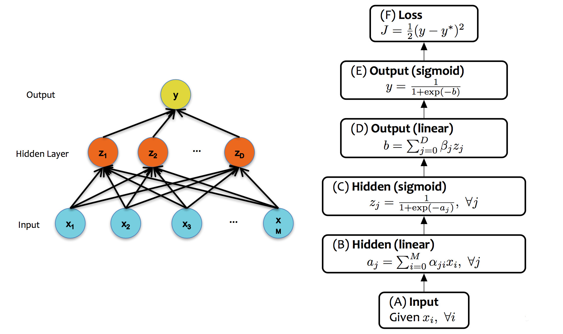
Now, suppose we have a training pair (\(\vec{x}, y)\). (That is, y is the correct class for \(\vec{x}\).) Updating the neural net weights happens as follows:

• Forward pass: starting from the input \(\vec{x}\), calculate the output values for all units. We work forwards through the network, using our current weights.
• Suppose the final output is \(y^*\). We put y and \(y^*\) into our loss function to calculate the final loss value.
• Backpropagation: starting from the loss at the end of the network and working backwards, calculate how changes to each weight will affect the loss. This combines the derivatives of each individual function with the values from the forward pass.

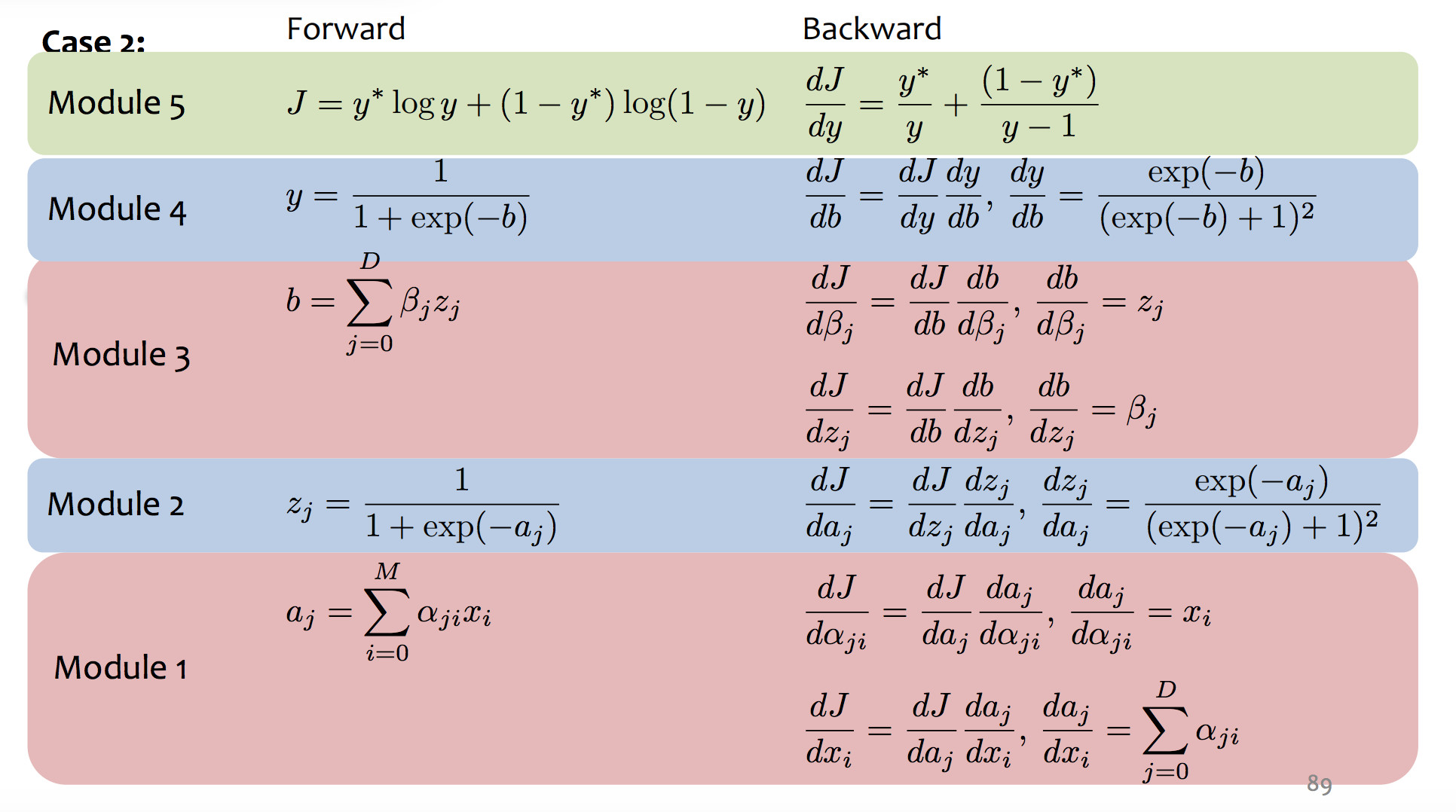
The diagram below shows the forward and backward values for our example network:

(from Matt Gormley)

Backpropagation is essentially a mechanical exercise in applying the chain rule repeatedly. Humans make mistakes, and direct manual coding will have bugs. So, as you might expect, computers have taken over most of the work as they for (say) register allocation. Read the very tiny example in Jurafsky and Martin (7.4.3 and 7.4.4) to get a sense of the process, but then assume you'll use TensorFlow or PyTorch to make this happen for a real network.

Three challenges in training

Unfortunately, training neural nets is somewhat of a black art because the process isn't entirely stable. Three issues are prominent:

• Symmetry breaking
• Overfitting
• Vanishing/exploding gradients

Symmetry Breaking

Perceptron training works fine with all weights initialized to zero. This won't work in a neural net, because each layer typically has many neurons connected in parallel. We'd like parallel units to look for complementary features but the naive training algorithm will cause them to have identical behavior. At that point, we might as well economize by just having one unit. Two approaches to symmetry breaking:

• Set the initial weights to random values.
• Randomize some aspect of the later training, e.g. ignore some randomly-chosen units on each update.

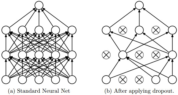
One specific proposal for randomization is dropout: Within the network, each unit pays attention to training data only with probability p. On other training inputs, it stops listening and starts reading its email or something. The units that aren't asleep have to classify that input on their own. This can help prevent overfitting.

from Srivastava et al.

Overfitting

Neural nets infamously tend to tune themselves to peculiarities of the dataset. This kind of overfitting will make them less able to deal with similar real-world data. The dropout technique will reduce this problem. Another method is "data augmentation".

Data augmentation tackles the fact that training data is always very sparse, but we have additional domain knowledge that can help fill in the gaps. We can make more training examples by perturbing existing ones in ways that shouldn't (ideally) change the network's output. For example, if you have one picture of a cat, make more by translating or rotating the cat. See this paper by Taylor and Nitschke.

Vanishing/exploding gradients

In order for training to work right, gradients computed during backprojection need to stay in a sensible range of sizes. A sigmoid activation function only works well when output numbers tend to stay in the middle area that has a significant slope.

• gradients too small: numbers can underflow, also training can become slow
• gradients too large: numbers can overflow

The underflow/overflow issues happen because numbers that are somewhat too small/large tend to become smaller/larger.

Several approaches to mitigating this problem, none of which looks (to me) like a solid, complete solution.

• ReLU units are less prone to these problems. However, they stop training if inputs force their outputs negative. So people often use a "leaky ReLU" function which has a very small slope on the negative side, e.g. f(x) = x for positive inputs, f(x) = 0.01x for negative ones.
• Initialize weights so that different layers end up with the same variance in gradients. For example, the variance may be set proportional to \(\frac{1}{N_{in}} \) or \(\frac{2}{N_{in} + N_{out}} \) where \(N_{in}\) is the number of incoming connections for this layer and \(N_{out}\) is the number of outgoing connections. There are several variants on this idea, e.g. Xavier and Kaiming initialization.
• Gradient clipping: detect excessively high gradients and reduce them.
• Weight regularization: many of the problematic situations involve excessively large weights. So add a regularization term to the network's loss function that measures the size of the weights (e.g. sum of the squares or magnitudes of the weights).

Notes

Credits to Matt Gormley are from 10-601 CMU 2017