(from Mark Hasegawa-Johnson, CS 440, Spring 2018)

Differentiable units

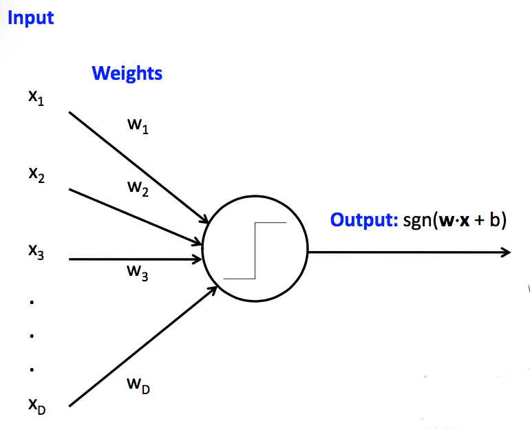
Classical perceptrons have a step function activation function, so they return only 1 or -1. Our accuracy is the count of how many times we got the answer right. When we generalize to multi-layer networks, it will be much more convenient to have a differentiable output function, so that we can use gradient descent to update the weights.

To do this, we need to separate two functions at the output end of the unit:

• the activation function: our model of uncertainty about the decision
• the loss function: the penalty for getting the decision wrong.

For the perceptron, the activation function is the sign function function: 1 if above the threshold, -1 if below it. The loss function for a perceptron is "zero-one loss". We get 1 for each wrong answer, 0 for each correct one.

So our whole classification function is the composition of three functions:

• the weighted sum of input feature values
• the activation function
• the loss function

In a multi-layer network, there will be activation functions at each layer and one loss function at the very end.

Activation Functions

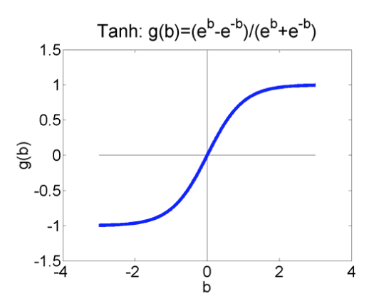
When we move to differentiable units for making neural nets, the popular choices for differentiable activation functions include the logistic (aka sigmoid), tanh, rectified linear unit (ReLu). Wikipedia has an excessively comprehensive list of alternatives.

The tanh function \( \frac{e^x - e^{-x}}{e^x + e^{-x}} \) looks like this:

from Mark Hasegawa-Johnson

The logistic/sigmoid function has equation \( \frac{1}{(1+e^{-x})} \). It is just like tanh, except rescaled so that it returns values between 0 and 1 (rather than between -1 and 1). The logistic form would be used when the designer wants to think of the values as probabilities (e.g. logistic regression). Otherwise one would choose whichever is more convenient for later stages of processing.

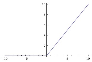
A rectified linear unit (ReLU) uses the function f, where f(x) = x when positive, f(x) = 0 if negative. It looks like this:

from Andrej Karpathy

The activation does not affect the decision from our single, pre-trained unit. Rather, the choice has two less obvious consequences:

• The output of the logistic function is in the right range to be interpreted as a probability, if that is desired.
• A slow transition across the decision boundary lets us treat values near the decision boundary as uncertain, both when training our unit and when feeding its value to later processing (e.g. in a neural net).

Loss Functions

Suppose that we have a training pair (x,y). So y is the correct output. Suppose that \(\hat{y}\) is the output of our unit (weighted average and then activation function). Popular differentiable loss functions include

• L2 norm: \((y-\hat{y})^2\)
• cross-entropy loss: \(-(y \log \hat{y} + (1-y)\log(1-\hat{y}))\)

In both cases, our goal is to minimize this loss averaged over all our training pairs.

When using the L2 norm to measure distances (e.g. in a 2D map), one would normally

• take the square of the difference for each individual coordinate (as shown above),
• add the squares up across all coordinates, and then
• take the square root of the result.

However, we're just trying to minimize the distance, not actually compute the distance. So we can skip the last (square root) step, because square root is monotonically increasing.

Recall that entropy is the number of bits required to (optimally) compress a pool of values. The high-level idea of cross-entropy is that we have built a model of probabilities (e.g. using some training data) and then use that model to compress a different set of data. Cross-entropy measures how well our model succeeds on this new data. This is one way to measure the difference between the model and the new data.

If you are curious, here is a longer list of loss functions.

Review: the chain rule

Remember the chain rule from calculus. If \(h(x) = f(g(x)) \), the chain rule says that \(h'(x) = f'(g(x))\cdot g'(x) \). In other words, to compute \(h'(x) \), we'll need the derivatives of the two individual functions, plus the value of of them applied to the input.

Example of differentiable updating

Let's assume we use the logistic/sigmoid for our activation function and the L2 norm for our loss function.

To work out the update rule for learning weight values, suppose we have a training example (x,y), where x is a vector of feature values. The output with our current weights is

\(\hat{y} = \sigma(w\cdot x)\) where \(\sigma\) is the sigmoid function.

Using the L2 norm as our loss function, our loss from just this one training sample is

\(L(w,x) = (y - \hat{y})^2\)

For gradient descent, we adjust our weights in the opposite of the gradient direction. That is, our update rule for one weight \(w_i\) should look like:

\( w_i = w_i - \alpha \cdot \frac{ \partial L(w,x)}{\partial w_i} \)

Let's figure out what \( \frac{ \partial L(w,x)}{\partial w_i} \) is. This requires some patience but is entirely mechanical. It's a calculation that you'll typically ask a software package (e.g. neural net utilities) to do for you.

\( \frac{ \partial L(w,x)}{\partial w_i} = \frac{ \partial (y - \hat{y})^2}{\partial w_i}\) (definition of L(w,x))
= \( 2(y-\hat{y}) \cdot \frac{\partial (y-\hat{y})}{\partial{w_i}} \) (chain rule)
= \( 2(y-\hat{y}) \cdot \frac{\partial (- \hat{y})}{\partial{w_i}} \) (y doesn't depend on \(w_i\)) = \( -2(y-\hat{y}) \cdot \frac{\partial \hat{y}}{\partial{w_i}} \) (y doesn't depend on \(w_i\))

OK, so now what is \(\frac{\partial \hat{y}}{\partial{w_i}} \)? If we look up the derivative of the sigmoid function, we find that \(\frac{\partial \sigma(z)}{\partial z} = \sigma(z)(1-\sigma(z))\). Using this fact:

\(\frac{\partial \hat{y}}{\partial{w_i}} \) = \(\frac{\partial \sigma(w\cdot x)}{\partial{w_i}} \) (definition of \(\hat{y}\))
= \(\sigma(w\cdot x)\cdot(1-\sigma(w\cdot x))\cdot\frac{\partial w\cdot x}{\partial w_i}\) (chain rule and the derivative of \(\sigma\))
= \(\sigma(w\cdot x)\cdot (1-\sigma(w\cdot x))\cdot x_i\) (it's just a polynomial)
= \(\hat{y}\cdot (1-\hat{y})\cdot x_i\) (definition of \(\hat{y}\))

Substituting this into our earlier formula, we get

\( \frac{ \partial L(w,x)}{\partial w_i} = -2\cdot (y-\hat{y})\cdot \hat{y}\cdot (1-\hat{y})\cdot x_i\)

So our update formula is

\( w_i = w_i + 2\alpha \cdot (y-\hat{y})\cdot \hat{y}\cdot (1-\hat{y})\cdot x_i\)

\(\alpha\) is just a tuning parameter, so we can fold 2 into it. This gives us our final update equation:

\( w_i = w_i + \alpha \cdot (y-\hat{y})\cdot \hat{y}\cdot (1-\hat{y})\cdot x_i\)

Ugly, unintuitive, but straightforward to code.