Basic perceptron

Recall that a linear classifier makes its decisions based on a linear combination of the input feature values. That is, if our input features values are \(x_1, x_2, \ldots, x_n\), it tests whether

\(w_1 x_1 + .... w_n x_n + b \ge 0\)

To avoid having to deal separately with the bias term b, we replace this with a fake feature \(x_0\) that is always set to 1, plus an additional weight \(w_0\). So then our decision equation becomes

\(w_0 x_0 + w_1 x_1 + .... w_n x_n \ge 0\)

Reformulating a bit further, let's pass this weighted sum through the sign function (sgn). We'll follow the neural net terminology and call this final function the "activation function." So then our classification is based on this test:

Is \(\text{sgn}(w_0 x_0 + w_1 x_1 + .... w_n x_n ) \) equal to 1 or -1?

We can make one of these units look like a neuron or a circuit component by drawing it like this:

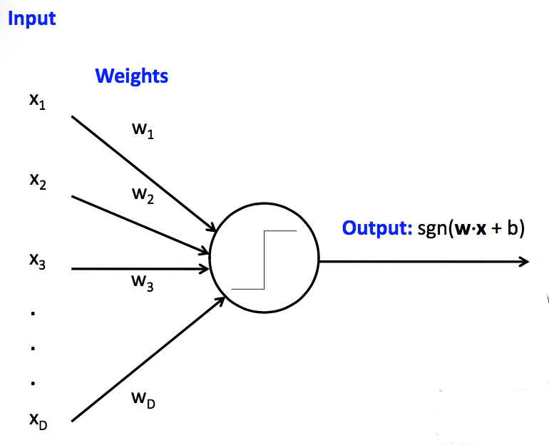(from Mark Hasegawa-Johnson, CS 440, Spring 2018)

This particular type of linear unit unit is called a perceptron. Perceptrons have limited capabilities but are particularly easy to train.

The training process

So far, we've assumed that the weights \(w_0,w_1,\ldots, w_n \) were given to us by magic. In practice, they are learned from training data. Suppose that we have a set T of training data pairs (x,y), where x is a feature vector and y is the (correct) class label. Our training algorithm looks like:

• Initialize weights \(w_0,\ldots, w_n\) to zero
• For each training example (x,y), update the weights to improve the changes of classifying x correctly.

Perceptron Learning Rule

Let's suppose that our unit is a classical perceptron, i.e. our activation function is the sign function. Then we can update the weights using the "perceptron learning rule". Suppose that x is a feature vector, y is the correct class label, and \(\hat{y}\) is the class label that was computed using our current weights. Then our update rule is:

• If \(\hat{y}\) = y, do nothing.
• Otherwise \(w_i = w_i + \alpha \cdot y \cdot x_i \)

The "learning rate" constant \(\alpha \) controls how quickly the update process changes in response to new data.

There's several variants of this equation, e.g.

\(w_i = w_i + \alpha \cdot (y-\hat{y}) \cdot x_i \)

When trying to understand why they are equivalent, notice that the only possible values for y and \(\hat{y}\) are 1 and -1. So if \( y = \hat{y} \), then \( (y-\hat{y}) \) is zero and our update rule does nothing. Otherwise, \( (y-\hat{y}) \) is equal to either 2 or -2, with the sign matching that of the correct answer (y). The factor of 2 is irrelevant, because we can tune \( \alpha \) to whatever we wish.

This training procedure will converge if

• data are linearly separable or
• we throttle the size of the updates as training proceeds by decreasing \(\alpha\).

Apparently convergence is guaranteed if the learning rate is proportional to \(\frac{1}{t}\) where t is the current iteration number. The book recommends a gentler formula: make \(\alpha \) proportional to \(\frac{1000}{1000+t}\).

Processing the training data

One run through training data through the update rule is called an "epoch." Training a linear classifier generally uses multiple epochs, i.e. the algorithm sees each training pair several times.

Datasets often have strong local correlations, because they have been formed by concatenating sets of data (e.g. documents) that each have a strong topic focus. So it's often best to process the individual training examples in a random order.

Limitations

Perceptrons can be very useful but have significant limitations.

• The decision boundary can only be a line.

  Fixes:

  • use multiple units (neural net)
  • massage input features to make the boundary linear

• If there is overlap between the two categories, the learning process can thrash between different boundary positions.

  Fixes:

  • reduce learning rate as learning progresses
  • don't update weights any more than needed to fix mistake in current example
  • cap the maximum change in weights (e.g. this example may have been a mistake)

• If there is a gap between the two categories, the training process may have trouble deciding where to place the boundary line.

  Fix: switch to a closely-related learning method called a "support vector machines" (SVM's). The big idea for an SVM is that only examples near the boundary matter. So we try to maximize the distance between the closest sample point and the boundary (the "margin").

Multi-class perceptrons

Perceptrons can easily be generalized to produce one of a set of class labels, rather than a yes/no answer. We use several parallel classifier units. Each has its own set of weights. Join the individual outputs into one output using argmax (i.e. pick the class that has the largest output value).

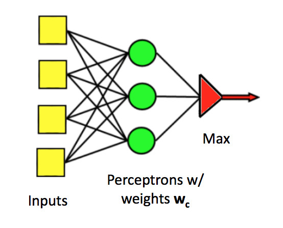(from Mark Hasegawa-Johnson, CS 440, Spring 2018)

Update rule: Suppose we see (x,y) as a training example, but our current output class is \(\hat{y}\). Update rule:

• Do nothing if y and \(\hat{y}\) are the same.
• Do nothing to the units for classes other than y and \(\hat{y}\).
• Each weight in class y: \(w_i = w_i + \alpha \cdot x_i \)
• Each weight in class \(\hat{y}\): \(w_i = w_i - \alpha \cdot x_i \)

The classification regions for a multi-class perceptron look like the picture below. That is, each pair of classes is separated by a linear boundary. But the region for each class is defined by several linear boundaries.

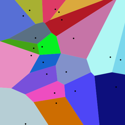from Wikipedia