Linear classifiers classify input items using a linear combination of feature values. Depending on the details, and the mood and theoretical biases of the author, a linear classifier may be known as
The variable terminology was created by the convergence of two lines of research. One (neural nets, perceptrons) attempts to model neurons in the human brain. The other (logistic regression, SVM) evolved from standard methods for linear regression.
A key limitation of linear units is that class boundaries must be linear. Real class boundaries are frequently not linear. So linear units typically
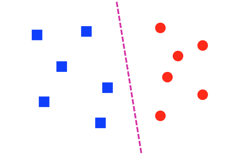
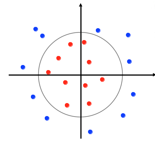
A dataset is linearly separable if we can draw a line (or, in higher dimensions, a hyperplane) that divides one class from the other. The lefthand dataset below is linearly separable; the righthand one is not.
 from Lana Lazebnik
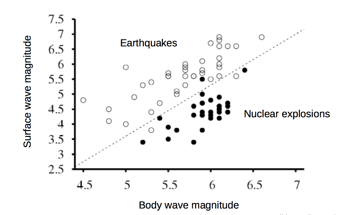
A common situation is that data may be almost linearly separable. That is, we can draw a line that correctly predicts the class for most of the data points, and we can't do any better by adjusting the line. That's often the best that can be done when the data is messy.
 from Lana Lazebnik
A single linear unit will try to separate the data with a line/hyperplane, whether or not the data really looks like that.
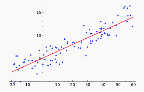
You've probably seen linear regression or, at least, used a canned function that performs it. However, you may well not remember what the term refers to. Linear regression is the process of fitting a linear function f to a set of (x,y) points. That is, we are given a set of data values \(x_i,y_i\). We stipulate that our model f must have the form \(f(x) = ax + b\). We'd like to find values for a and b that minimize the distance between the \(f(x_i)\) and \(y_i\), averaged over all the datapoints. For example, the red line in this figure shows the line f that approximates the set of blue datapoints.
 From Wikipedia
There are two common ways to "measure the distance between \(f(x_i)\) and \(y_i\)":
The popular "least squares" method uses the L2 norm. Because this error function is a simple differentiable function of the input, there is a well-known analytic solution for finding the minimum. (See the textbook or many other places.) There are also so-called "robust" methods that minimize the L1 norm. These are a bit more complex but less sensitive to outliers (aka bad input values).
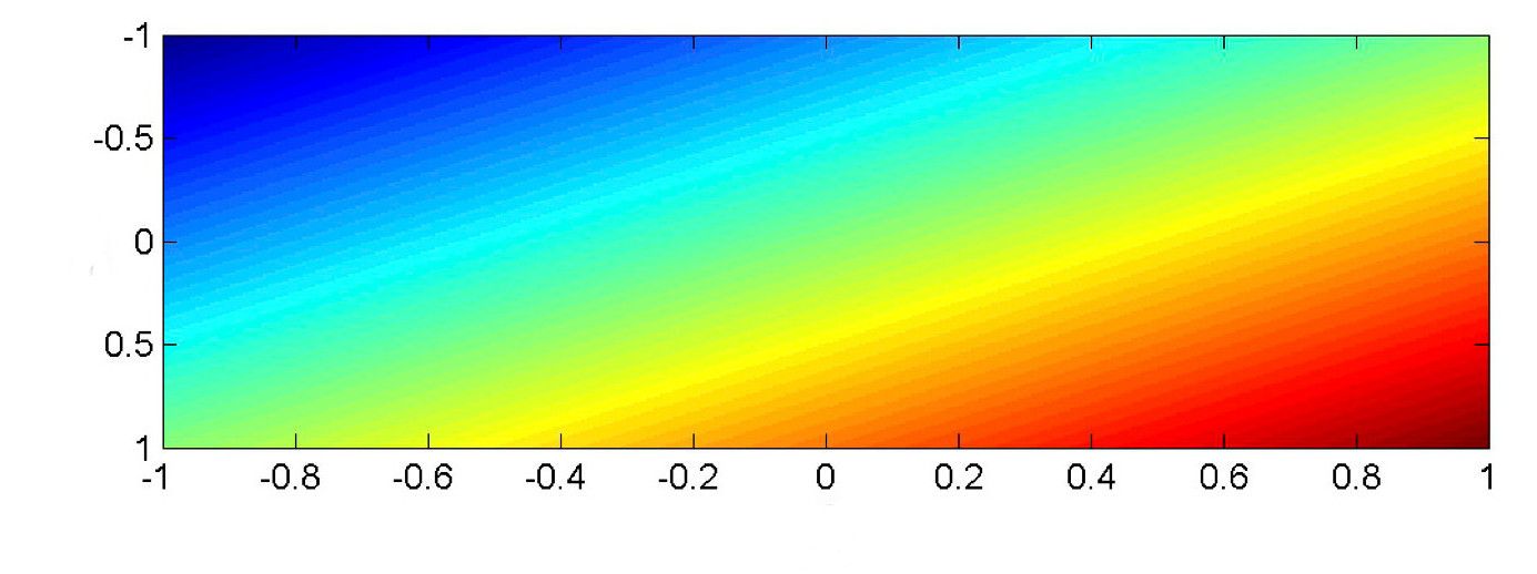
In most classification tasks, our input values are a vector \(\vec{x}\). Suppose that \(\vec{x}\) is two-dimensional, so we're fitting a model function \(f(x_1,x_2)\). A linear function of two input variables must look as follows, where color shows values of the output value \(f(x_1,x_2)\). (red high to blue low).
 from Mark Hasegawa-Johnson, CS 440, Spring 2018
In classification, we will typically be comparing the output value \(f(x_1,x_2)\). against a threshold T. In this picture, \(f(x_1, x_2) =T\) is a color contour. E.g. perhaps it's the middle of the yellow stripe. The division boundary (i.e. \(f(x_1,x_2) = T\)) is always linear: a straight line for a 2D input, a plane for inputs of higher dimension.
The basic set-up for a linear classifier is shown below. Look at only one class (e.g. pink for cat). Each input example generates a feature vector (x). The four pixel values \(x_1, x_2, x_3, x_4 \) are multiplied by the weights for that class (e.g. the pink cells) to produce a score for that class. A bias term (b) is added to produce the weighted sum \(w_1 x_1 + .... w_n x_n + b \).
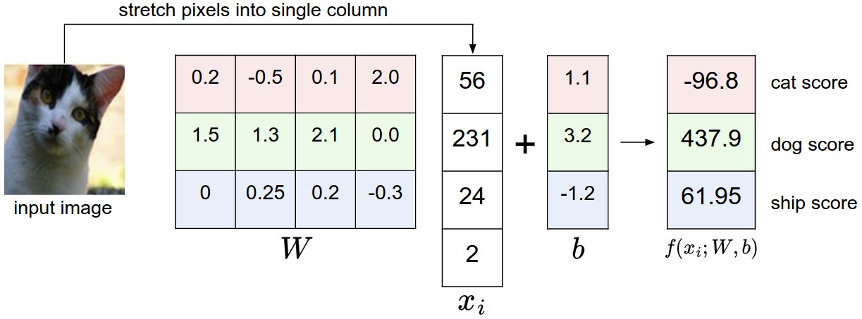
(from Andrej Karpathy cs231n course notes via Lana Lazebnik)
In this toy example, the input features are are individual pixel values. In a real working system, they would probably be something more sophisticated, such as SIFT features or the output of an early stage of neural processing. In a text classifcation task, one might use word or bigram probabilities.
To make a multi-way decision (as in this example), we compare the output values for several classes and pick the class with the highest value. In this toy example, the algorithm makes the wrong choice (dog). Clearly the weights \(w_i\) are key to success.
To make a yes/no decision, we compare the weighted sum to a threshold. The bias term adjusts the output so that we can use a standard threshold: 0 for neural nets and 0.5 for logistic regression. (We'll assume we want 0 in what follows.) In situations where the bias term is notationally inconvenient, we can make it disappear (superficially) by introducing a new input feature \(x_0\) which is tied to the constant 1. Its weight \(w_0\) is the bias term.
In Naive Bayes, we fed a feature vector into a somewhat similar equation (esp. if you think about everything in log space). What's different here?
First, the feature values in Naive Payes were probabilities. E.g. a single number might be the probability of seeing the word "elephant" in some type of text. The values here are just numbers, not in the range [0,1]. We don't know whether all of them are on the same scale.
In naive Bayes, we assumed that features were conditionally independent, given the class label. This may be a reasonable approximation for some sets of features, but it's frequently wrong enough to cause problems. For example, in a bag of words model, "San" and "Francisco" do not occur independently even if you know that the type of text is "restaurant reviews." Logistic regression (a natural upgrade for naive Bayes) allows us to handle features that may be correlated. For example, the individual weights for "San" and "Francisco" can be adjusted so that the pair's overall contribution is more like that of a single word.