a real-world trellis (supporting a passionfruit vine)
Once we have estimated the model parameters, the Viterbi algorithm finds the highest-probability tag sequence for each input word sequence. Suppose that our input word sequence is \(w_1,\ldots w_n\).
The basic data structure is an n by m array (v), where n is the length of the input word sequence and m is the number of different (unique) tags. Each cell (k,t) in the array contains the probability v(k,t) of the best sequence of tags for \(w_{1}\ldots w_{k} \) that ends with tag t. We also store b(k,t), which is the previous tag in that best sequence. This data structure is called a "trellis."
The Viterbi algorithm fills the trellis from left to right, as follows:
Initialization: We fill the first column using the initial probabilities. Specifically, the cell for tag t gets the value \( v(1,t) = P_S (t) * P_E(w_1 \mid t) \).
Moving forwards in time: Use the values in column k to fill column k+1. Specifically
For each tag \(tag_B\)That is, we compute \(v(k, tag_A) * P_T(tag_B \mid tag_A) * P_E(w_{k+1} \mid tag_B) \) for all possible tags \(tag_A\). The maximum value goes into trellis cell \( v(k+1,tag_B) \) and the corresponding value of \(tag_A\) is stored in \( b(k+1,tag_B) \).\( v(k+1,tag_B) = \max_{tag_A}\ \ v(k, tag_A) * P_T(tag_B \mid tag_A) * P_E(w_{k+1} \mid tag_B) \)
\( b(k+1,tag_B) = \text{argmax}_{tag_A}\ \ v(k, tag_A) * P_T(tag_B \mid tag_A) * P_E(w_{k+1} \mid tag_B) \)Finishing: When we've filled the entire trellis, pick the best tag B in the final (time=n) column. Trace backwards from B, using the values in b, to produce the output tag sequence.
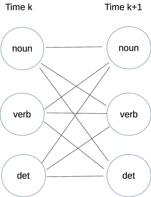
Here's a picture of one section of the trellis, drawn as a graph. A path ending in some specific tag at time k might continue to any one of the possible tags at time k+1. So each cell in column k is connected to all cells in column k+1. The name "trellis" comes from this dense pattern of connections between each timestep and the next.
The Viterbi algorithm depends on this mystery rule for computing a value at time k+1 from a value at time k.
\( v(k+1,tag_b) \ = \ v(k,tag_a) * P_T(tag_b \mid tag_a) * P_E(w_{k+1} \mid tag_b) \)
What is it?
This about searching the trellis like a maze, but consistently moving from left to right (i.e. following the progression of time). The righthand side of our equation is the product of two terms:
As we move through the trellis, we're multiplying costs, where we would add them in a normal maze. But the rest of the method is similar. And we produce the final output path by tracing backwards, just as we would in a maze search algorithm.
The probabilities in the Viterbi algorithm can get very small, creating a real possibility of underflow. So the actual implementation needs to convert to logs and replace multiplication with addition. After the switch to addition, the Viterbi computation looks even more like edit distance or maze search. That is, each cell contains the cost of the best path from the start to our current timestep. As we move to the next timestep, we're adding some additional cost to the path. However, for Viterbi we prefer larger, not smaller, values.
The asymptotic running time for this algorithm is \( O(m^2 n) \) where n is the number of input words and m is the number of different tags. In typical use, n would be very large (the length of our test set) and m fairly small (e.g. 36 tags in the Penn treebank). Moreover, the computation is quite simple. So Viterbi ends up with good constants and therefore a fast running time in practice.
The Viterbi algorithm can be extended in several ways. First, high accuracy taggers typically use two tags of context to predict each new tag. This increases the height of our trellis from m to \(m^2\). So the full trellis could become large and expensive to computer. These methods typically use beam search, i.e. keep only the most promising trellis states for each timestep.
So far, we've been assuming that all unseen words should be treated as unanalyzable unknown objects. However, the form of a word often contains strong cues to its part of speech. For example, English words ending in "-ly" are typically adverbs. Words ending in "-ing" are either nouns or verbs. We can use these patterns to make more accurate guesses for emission probabilities of unseen words.
Finally, suppose that we have only very limited amounts of tagged training data, so that our estimated model parameters are not very accurate. We can use untagged training data to refine the model parameters, using a technique called the forward-backward (or Baum-Welch) algorithm. This is an application of a general method called "Expectation Maximization" (EM) and it iteratively tunes the HMM's parameters so as to improve the computed likelihood of the training data.
Here is an interesting example from 1980 of how an HMM can automatically learn sound classes: R. L. Cave and L. P. Neuwirth, "Hidden Markov models for English."