a real-world trellis (supporting a passionfruit vine)

Recap

In an HMM, we have a sequence of tags at the top. Each tag depends only on the previous tag. Each word (bottom row) depends only on the corresonding tag.

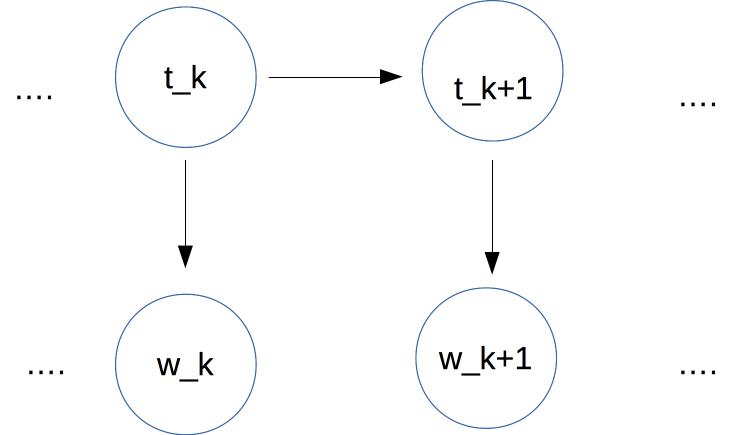
At each time position k, we assume that

\(P(w_k)\) depends only on \(P(t_k)\)
\(P(t_k) \) depends only on \(P(t_{k-1})) \)

Given an input word sequence W, our goal is to find the tag sequence T that maximizes

\( P (T \mid W)\)
\(\propto P(W \mid T) * P(T) \)
\( = \prod_{i=1}^n P(w_i \mid t_i)\ \ * \ \ P(t_1 \mid \text{START})\ \ *\ \ \prod_{k=2}^n P(t_k \mid t_{k-1}) \)

Let's label our probabilities as \(P_S\), \(P_E\), and \(P_T\) to make their roles more explicit. Using this notation, we're trying to maximize

\( \prod_{i=1}^n P_E(w_i \mid t_i)\ \ * \ \ P_S(t_1)\ \ *\ \ \prod_{k=2}^n P_T(t_k \mid t_{k-1}) \)

So we need to estimate three types of parameters:

• \( P_S(t_1) \) initial probabilities
• \( P_T(t_k | t_{k-1}) \) transition probabilities
• \( P_E(w_i | t_i) \) emission probabilities

Toy model

For simplicity, let's assume that we have only three tags: Noun, Verb, and Determiner (Det). Our input will contain sentences that use only those types of words, e.g.

    Det Noun     Verb    Det Noun   Noun
    The student  ate     the ramen  noodles

    Det Noun   Noun  Verb    Det Noun
    The maniac rider crashed his bike.

We can look up our initial probabilities, i.e. the probability of various values for \(P_S(t_1)\) in a table like this.

tag	\(P_S(tag)\)
Verb	0.01
Noun	0.18
Det	0.81

We can estimate these by counting how often each tag occurs at the start of a sentence in our training data.

Transition probabilities

In the (correct) tag sequence for this sentence, the tags \(t_1\) and \(t_5\) have the same value Det. So the possibilities for the following tags (\(t_2\) and \(t_6\)) should be similar. In POS tagging, we assume that \(P_T(t_{k+1} \mid t_k)\) depends only on the identities of \(t_{k+1}\) and \( t_k\), not on their time position k. (This is a common assumption for Markov models.)

This is not an entirely safe assumption. Noun phrases early in a sentence are systematically different from those toward the end. The early ones are more likely to be pronouns or short noun phrases (e.g. "the bike"). The later ones more likely to contain nouns that are new to the conversation and, thus, tend to be more elaborate (e.g. "John's fancy new racing bike"). However, abstracting away from time position is a very useful simplifying assumption which allows us to estimate parameters with realistic amounts of training data.

So, suppose we need to find a transition probability \( P_T(t_k | t_{k-1}) \) for two tags \(t_{k-1} \) and \(t_k \) in our tag sequence. We consider only the identities of the two tags, e.g. \(t_{k-1} \) might be DET and \(t_k \) might be NOUN. And we look up the pair of tags in a table like this

	Next Tag
Previous tag	Verb	Noun	Det
Verb	0.02	0.21	0.77
Noun	0.51	0.44	0.05
Det	\(\approx 0 \)	0.99	0.01

We can estimate these by counting how often a 2-tag sequence (e.g. Det Noun) occurs and dividing by how often the first tag (e.g. Det) occurs.

Notice the near-zero probability of a transition from Det to Verb. If this is actually zero in our training data, do we want to use smoothing to fill in a non-zero number? Yes, because even "impossible" transitions may occur in real data due to typos or (with larger tagsets) very rare tags. Laplace smoothing should work well.

Finite-state automaton

We can view the transitions between tags as a finite-state automaton (FSA). The numbers on each arc is the probability of that transition happening.

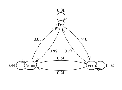
These are conceptually the same as the FSA's found in CS theory courses. But beware of small differences in conventions.

• You can start in any state (probability given by the initial probability table).
• A transition always exists between every pair of states, but each transition has an associated probability of happening.
• Output (words) is generated when you enter a state, not on the transition between states.

Emission probabilities

Our final set of parameters are the emission probabilities, i.e. \(P_E(w_k | t_k)\) for each position k in our tag sequence. Suppose we have a very small vocabulary of nouns and verbs to go with our toy model. Then we might have probabilities like

   Verb   played 0.01
          ate   0.05
          wrote 0.05
          saw   0.03
          said  0.03
          tree  0.001
      
   Noun  boy   0.01
         girl  0.01
         cat   0.02
         ball  0.01
         tree  0.01
         saw   0.01

   Det  a    0.4
        the  0.4
        some 0.02
        many 0.02

Because real vocabularies are very large, it's common to see new words in test data. So it's essential to smooth, i.e. reserve some of each tag's probability for

• new words
• familiar words seen with a new tag

However, the details may need to depend on the type of tag. Tags divide (approximately) into two types

• open class, aka content words (e.g. verbs, nouns, adjectives)
• closed class, aka function words (e.g. prepositions, determiners)

It's very common to see new open-class words. In English, open-class tags for existing words are also likely, because nouns are often repurposed as verbs, and vice versa. E.g. the proper name MacGyver spawned a verb, based on the improvisational skills of the TV character with that name. So open class tags need to reserve significant probability mass for unseen words, e.g. larger Laplace smoothing constant. It's much less common to encounter new closed-class words, e.g. a new conjunction. So these tags should have a smaller Laplace smoothing constant. The amount of probability mass to reserve for each tag can be estimated by looking at the tags of "hapax" words (words that occur only once) in our training data.