For each variable X, maintain set D(X) containing all possible values for X.
Run DFS. At each search step:
And we saw some heuristics for choosing variables and values in step 1.
When we assign a value to variable X, forward checking only checks variables that share a constraint with X, i.e. are adjacent in the constraint graph. This is helpful, but we can do more to exploit the constraints. Constraint propagation works its way outwards from X's neighbors to their neighbors, continuing until it runs out of nodes that need to be updated.
Suppose we are coloring the same state graph with {Red,Green,Blue} and we decide to first color New Hampshire red:
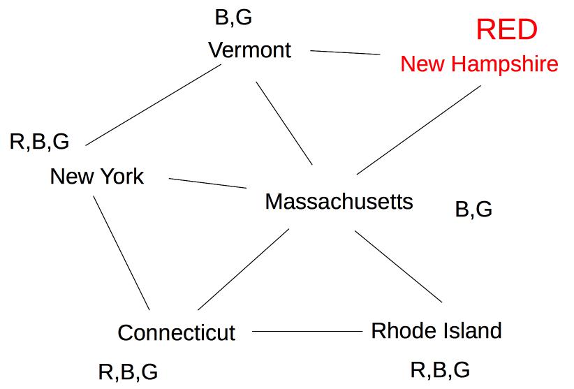
Forward checking then removes Red from Vermont and Massachusetts. Suppose we now color New York Green. Forward checking removes Green from its immediate neighbors, giving us this:
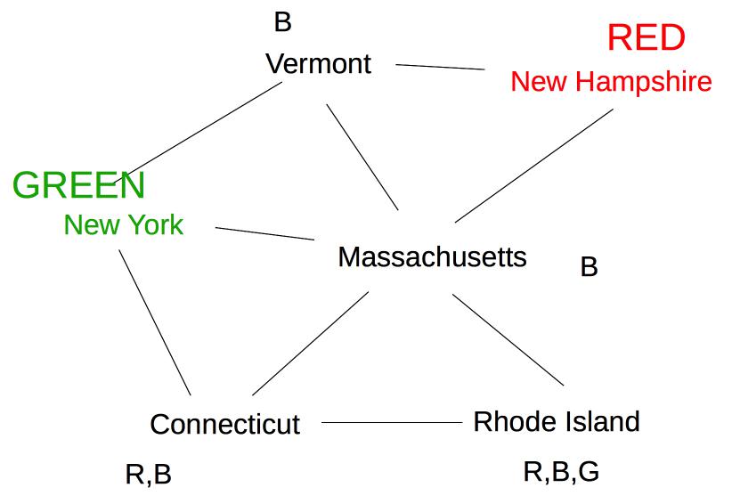
At this point, forward checking stops. Constraint propagation continues. Since Massachusetts now has fewer possible values, its neighbor Connecticut also needs to be updated.
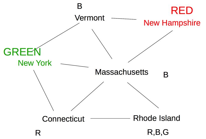
Rhode Island is adjacent to Massachusetts and Connecticut, so its options need to be updated:
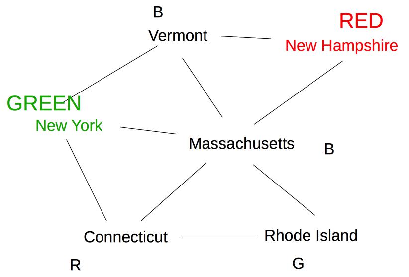
Finally, Vermont is a neighbor of Massachusetts, so update its options.
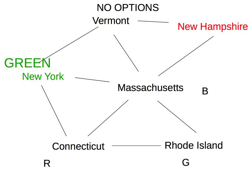
Since this leaves Vermont with no possible values, we backtrack to our last decision point (coloring New York Green).
The exact sequence of updates depends on the order in which we happen to have stored our nodes. However, constraint propagation typically makes major reductions in the number of options to be explored, and allows us to figure out early that we need to backtrack.
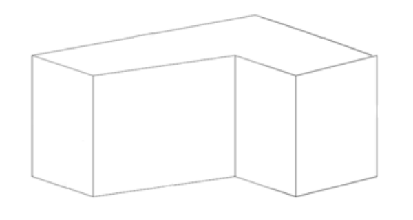
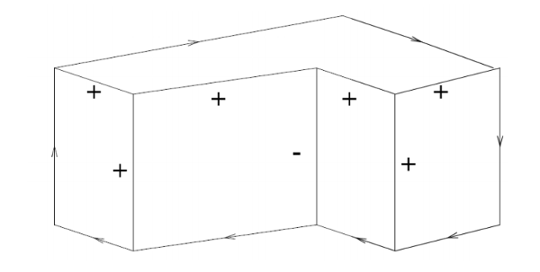
Constraint propagation was developed by David Waltz in the early 1970's for the Shakey project (e.g. see David Waltz's 1972 thesis). The original task was to take a wireframe image of blocks and decorate each edge with a labels indicating its type. Object boundaries are indicated by arrows, which need to point clockwise around the bounary. Plus and minus signs mark internal edges that are convex and concave.
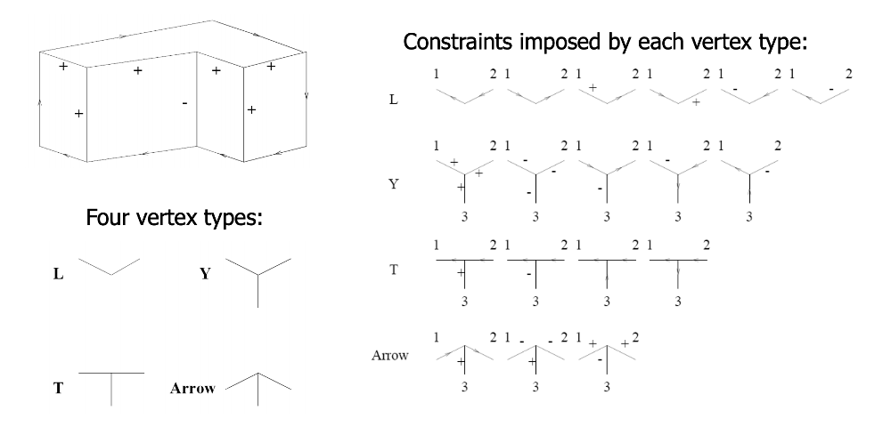
In this problem, the constraints are provided by the vertices. Each vertex is classified into one of four types, based on the number of edges and their angles. For each type, there are only a small set of legal ways to label the incoming edges.
See this contemporary video of the labeller in action.
Because line labelling has strong local constraints, constraint propagation can sometimes nail down the exact solution without any search. A more typical situation is that we need to use a combination of backtracking search and constraint propagation. Constraint propagation can be added at two points in our backtracking search:
It takes a bit of care to implement constraint propagation correctly. We'll look at the AC-3 algorithm, developed by David Waltz and Alan Mackworth (1977).
The constraint relationship between two variables ("some constraint relates the values of X and Y") is symmetric. For this algorithm, however, we will treat constraints between variables ("arcs") as ordered pairs. So the pair (X,Y) will represent contraint flowing from Y to X.
The function Revise(X,Y) prunes values from D(X) that are inconsistent with what's currently in D(Y).
The main datastructure in AC-3 is a queue of pairs ("arcs") that still need attention.
Given these definitions, AC-3 works like this:
Initialize queue. Two options
- all constraint arcs in problem [for starting up a new CSP search]
- all arcs (X,Y) where Y's value was just set [for use during CSP search]
Loop:
- Remove (X,Y) from queue. Call Revise(X,Y).
- If D(X) has become empty, halt returning a value that forces main algorithm to backtrack.
- If D(X) has been changed (but isn't empty), push all arcs (C,X) onto the queue. Exception: don't push (Y,X).
Stop when queue is empty
Near the end of AC-3, we push all arcs (C,X) onto the queue, but we don't push (Y,X). Why don't we need to push (Y,X)?
Do attempt to solve this yourself first. It will help you internalize the details of the AC-3 algorithm. Then have a look at the solution.
See the CSPLib web page for more details and examples.