A decision tree makes its decision by asking a series of questions. For example, here is a a decision tree user interface for identifying vines (by Mara Cohen, Brandeis University). The features, in this case, are macroscopic properties of the vine that are easy for a human to determine, e.g. whether it has thorns. The top levels of this tree look like
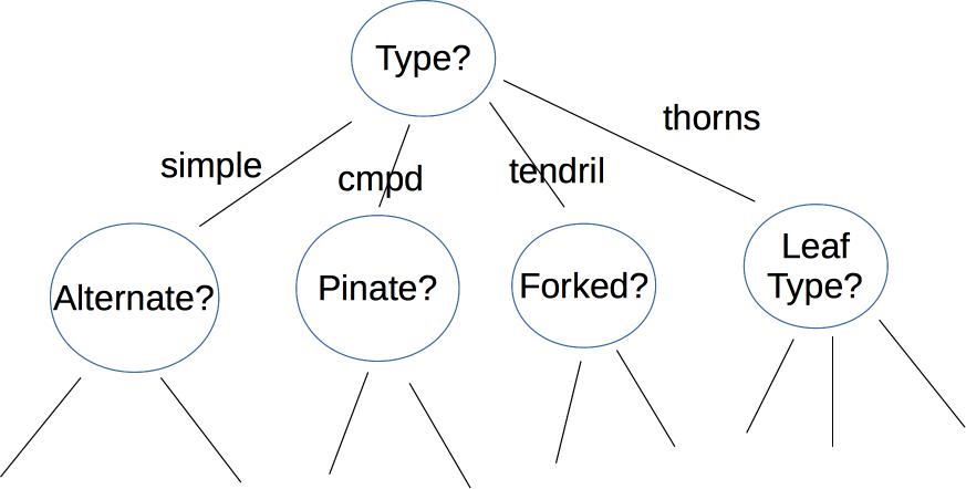
Depending on the application, the nodes of the tree may ask yes/no questions, multiple choice (e.g. simple vs. complex vs. tendril vs thorns), or set a threshold on a continuous space of values (e.g. is the tree below or above 6' tall?). The output label may be binary (e.g. is this poisonous?), from a small set (edible, other non-poisonous, poisonous), or from a large set (e.g. all vines found in Massachusetts). The strength of decision trees lies in this ability to use a variety of different sorts of features, not limited to well-behaved numbers.
Here's an example of a tree created by thresholding two continuous variable values (from David Forsyth, Applied Machine Learning). Notice that the split on the second variable (x) is different for the two main branches.
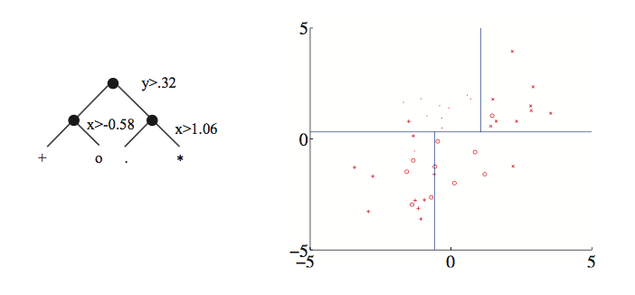
Each node in the tree represents a pool of examples. Ideally, each leaf node contains only objects of the same type. However, that isn't always true if the classes aren't cleanly distinguished by the available features (see the vowel picture above). So, when we reach a leaf node, the algorithm returns the most frequent label in its pool.
If we have enough decision levels in our tree, we can force each pool to contain objects of only one type. However, this is not a wise decision. Deep trees are difficult to construct (see the algorithm in Russell and Norvig) and prone to overfitting their training data. It is more effective to create a "random forest", i.e. a set of shallow trees (bounded depth) and have these trees vote on the best label to return. The set of shallow trees is created by choosing variables and possible split locations randomly.
Whether we're building a deep or shallow tree, some possible splits are a bad idea. For example, the righthand split leaves us with two half-size pools that are no more useful than the original big pool.
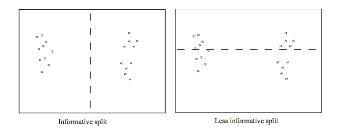
From David Forsyth, Applied Machine Learning.
A good split should produce subpools that are less diverse than the original pool. If we're choosing between two candidate splits (e.g. two thresholds for the same numerical variable), it's better to pick the one that produces subpools that are more uniform. Diversity/uniformity is measured using entropy.
Suppose that we are trying to compress English text, by translating each character into a string of bits. We'll get better compression if more frequent characters are given shorter bit strings. For example, the table below shows the frequencies and Huffman codes for letters in a toy example from Wikipedia.
| Char | Freq | Code | Char | Freq | Code | Char | Freq | Code | Char | Freq | Code | Char | Freq | Code | Char | Freq | Code | Char | Freq | Code |
|---|---|---|---|---|---|---|---|---|---|---|---|---|---|---|---|---|---|---|---|---|
| space | 7 | 111 | a | 4 | 010 | e | 4 | 000 | ||||||||||||
| f | 3 | 1101 | h | 2 | 1010 | i | 2 | 1000 | m | 2 | 0111 | n | 2 | 0010 | s | 2 | 1011 | t | 2 | 0110 |
| l | 1 | 11001 | o | 1 | 00110 | p | 1 | 10011 | r | 1 | 11000 | u | 1 | 00111 | x | 1 | 10010 |
Suppose that we have a (finite) set of letter types S. Suppose that M is a finite list of letters from S, with each letter type (e.g. "e") possibly included more than once in M. Each letter type c has a probability P(c) (i.e. its fraction of the members of M). An optimal compression scheme would require \(\log(\frac{1}{P(c)}) \) bits in each code. (All logs in this discussion are base 2.)
To understand why this is plausible, suppose that all the characters have the same probability. That means that our collection contains \(\frac{1}{P(c)} \) different characters. So we need \(\frac{1}{P(c)} \) different codes, therefore \(\log(\frac{1}{P(c)}) \) bits in each code. For example, suppose S has 8 types of letter and M contains one of each. Then we'll need 8 distinct codes (one per letter), so each code must have 3 bits. This squares with the fact that each letter has probability 1/8 and \(\log(\frac{1}{P(c)}) = \log(\frac{1}{1/8}) = \log(8) = 3 \).
The entropy of the list M is the average number of bits per character when we replace the letters in M with their codes. To compute this, we average the lengths of the codes, weighting the contribution of each letter c by its probability P(c). This give us
\( H(M) = \sum_{c \in S} P(c) \log(\frac{1}{P(c)}) \)
Recall that \(\log(\frac{1}{P(c)}) = -\log(P(c))\). Applying this, we get the standard form of the entropy definition.
\( H(M) = - \sum_{c \in S} P(c) \log(P(c)) \)
In practice, good compression schemes don't operate on individual characters and also they don't achieve this theoretical optimum bit rate. However, entropy is a very good way to measure the homogeneity of a collection of discrete values, such as the values in the decision tree pools.
For more information, look up Shannon's source coding theorem.