Recall: a classifier maps input examples (each a set of feature values) to class labels. Our task is to train a model on a set of examples with labels, and then assign the correct labels to new input examples.
Here's a schematic representation of English vowels (from Wikipedia). From this, you might reasonable expect to experimental data to look like several tight clusters of points, well-separated. If that were true, then classification would be easy: model each cluster with a regeion of simple shape (e.g. ellipse), compare a new sample to these region, and pick the one that contains it.
However, experimental datapoints for these vowels (even after some normalization) actually look more like the following. If we can't improve the picture by clever normalization (sometimes possible), we need to use more robust methods of classification.
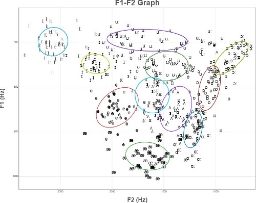
(These are the tirst two formants of English vowels by 50 British speakers, normalized by the mean and standard deviation of each speaker's productions. From the Experimental Phonetics course PALSG304 at UCL.)
Another way to classify an input example is to find the most similar training example and copy its label.
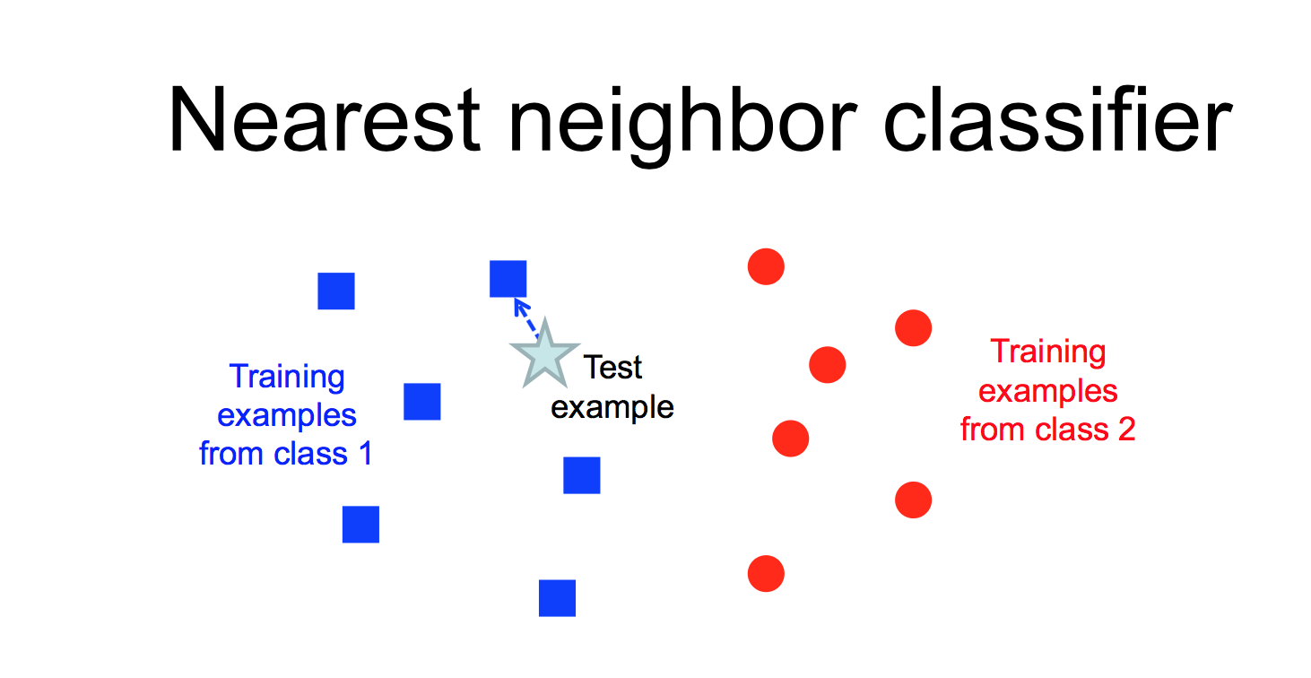 from Lana Lazebnik
This "nearest neighbor" method is prone to overfitting, especially if the data is messy and so examples from different classes are somewhat intermixed. However, performance can be greatly improved by finding the k nearest neighbors for some small value of k (e.g. 5-10).
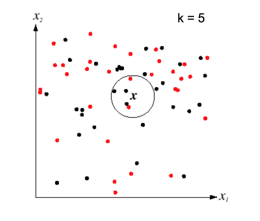 from Lana Lazebnik
K nearest neighbors can model complex patterns of data, as in the following picture. Notice that larger values of k smooth the classifier regions, making it less likely that we're overfitting to the training data.
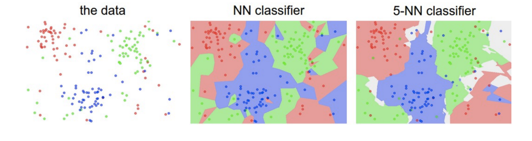 from Andrej Karpathy
A limitation of k nearest neighbors is that the algorithm requires us to remember all the training examples, so it takes a lot of memory if we have a lot of training data. Moreover, the obvious algorithm for classifying an input image X requires computing the distance from X to every stored image. In low dimensions, a k-D tree can be used to find efficiently find the nearest neighbors for an input example. However, efficiently handling higher dimensions is more tricky and beyond the scope of this course.
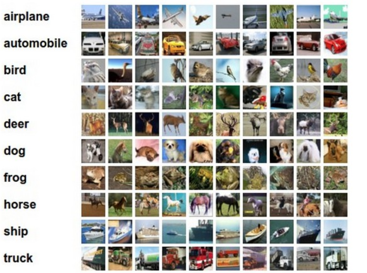
This method can be applied to somewhat more complex types of examples. Consider the CFAR-10 dataset below. (Pictures are from Andrej Karpathy cs231n course notes.) Each image is 32 by 32, with 3 color values at each pixel. So we have 3072 feature values for each example image.
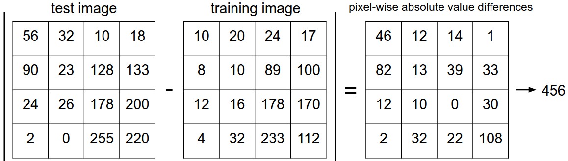
We can calculate the distance between two examples by subtracting corresponding feature values. Here is a picture of how this works for a 4x4 toy image.
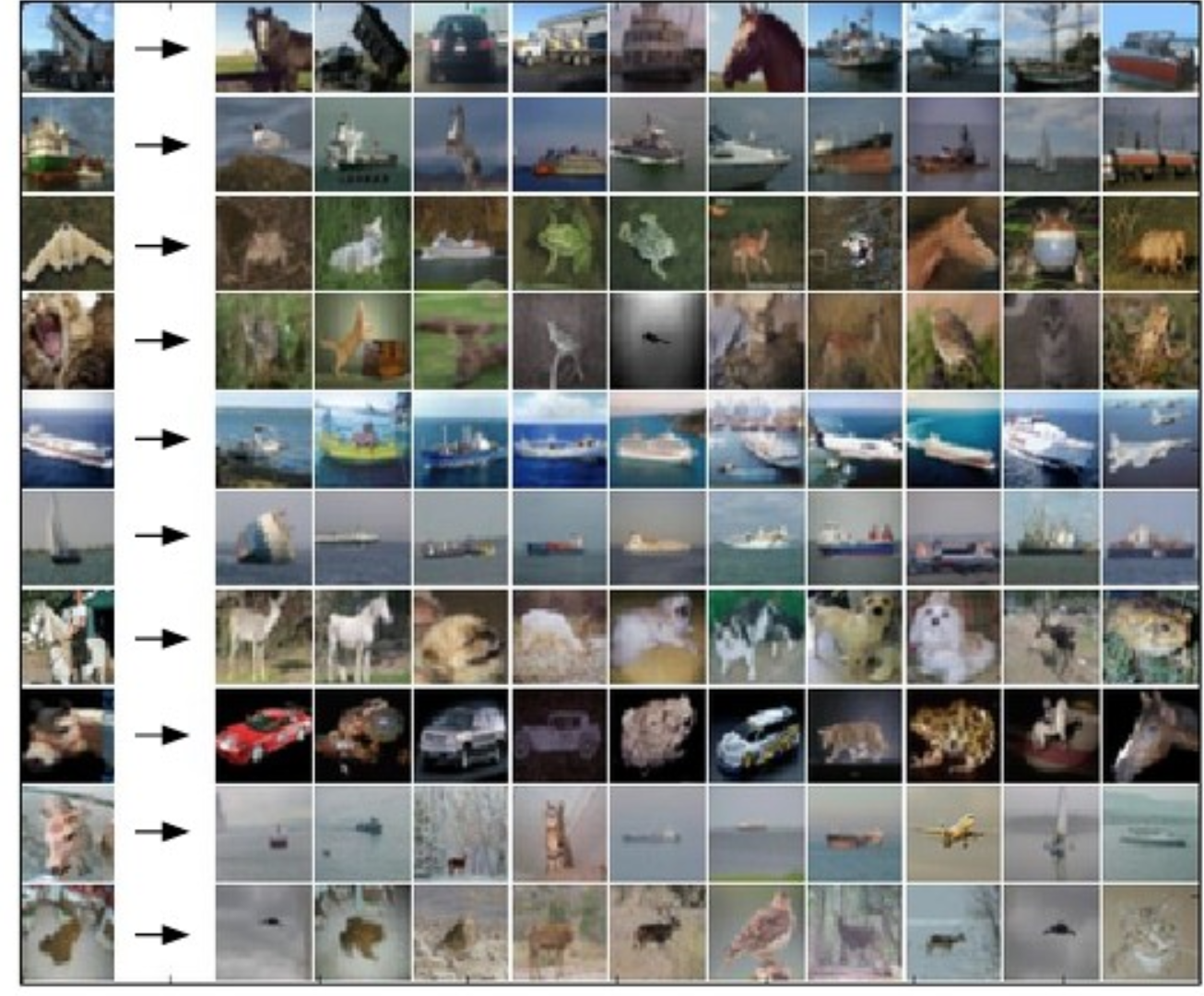
The following picture shows how some sample test images map to their 10 nearest neighbors.
More precisely, suppose that \(\vec{x}\) and \(\vec{y}\) are two feature vectors (e.g. pixel values for two images). Then there are two different simple ways to calculate the distance between two feature vectors:
As we saw with A* search for robot motion planning, the best choice depends on the details of your dataset. The L1 norm is less sensitive to outlier values. The L2 norm is continuous and differentiable, which can be handy for certain mathematical derivations.
