 Armadillo (picture from
Prairie Rivers Network)
Armadillo (picture from
Prairie Rivers Network)
Recall our document classification problem. Our input document is a string of words (perhaps not all identical) \( W_1, ..., W_n \)
Suppose that we have cleaned up our words, as discussed in the last video and now we're trying to label input documents as either CLA or CLB. To classify the document, our naive Bayes, bag of words model, compares these two values:
\( P(\text{CLA}) * \prod_{k=1}^n P(W_k | \text{CLA} ) \)
\( P(\text{CLB}) * \prod_{k=1}^n P(W_k | \text{CLB})\)
We need to estimate the parameters P(W | CLA) and P(W | CLB) for each word type W.
Now, let's look at estimating the probabilities. Suppose that we have a set of documents from a particular class C (e.g. CLA English) and suppose that W is a word type. We can define:
count(W) = number of times W occurs in the documents
n = number of total words in the documents
A naive estimate of P(W|C) would be \(P(W | \text{C}) = \frac{\text{count}(W)}{n}\). This is not a stupid estimate, but a few adjustments will make it more accurate.
The probability of most words is very small. For example, the word "Markov" is uncommon outside technical discussions. (It was mistranscribed as "mark off" in the original Switchboard corpus.) Worse, our estimate for P(W|C) is the product of many small numbers. Our estimation process can produce numbers too small for standard floating point storage.
To avoid numerical problems, researchers typically convert all probabilities to logs. That is, our naive Bayes algorithm will be maximizing
\(\log(P(\text{C} | W_1,\ldots W_k))\ \ \propto \ \ \log(P(\text{C})) + \sum_{k=1}^n \log(P(W_k | \text{C}) ) \)
Notice that when we do the log transform, we need to replace multiplication with addition.
Recall that we train on one set of documents and then test on a different set of documents. For example, in the Boulis and Ostendorf gender classifcation experiment, there were about 14M words of training data and about 3M words of test data.
Training data doesn't contain all words of English and is too small to get a representative sampling of the words it contains. So for uncommon words:
Smoothing assigns non-zero probabiities to unseen words. Since all probabilities have to add up to 1, this means we need to reduce the estimated probabilities of the words we have seen. Think of a probability distribution as being composed of stuff, so there is a certain amount of "probability mass" assigned to each word. Smoothing moves mass from the seen words to the unseen words.
Questions:
Some unseen words might be more likely than others, e.g. if it looks like a legit English word (e.g. boffin) it might be more likely than something using non-English characters (e.g. bête).
Smoothing is critical to the success of many algorithms, but current smoothing methods are witchcraft. We don't fully understand how to model the (large) set of words that haven't been seen yet, and how often different types might be expected to appear. Popular standard methods work well in practice but their theoretical underpinnings are suspect.
Laplace smoothing is a simple technique for addressing the problem:
All unseen words are represented by a single word UNK. So the probability of UNK should represent all of these words collectively.
n = number of words in our Class C training data
count(W) = number of times W appeared in Class C training data
To add some probability mass to UNK, we increase all of our estimates by \( \alpha \), where \(\alpha\) is a tuning constant between 0 and 1 (typically small). So our probabilities for UNK and for some other word W are:
P(UNK | C) = \(\alpha \over n\)
P(W | C) = \({count(W) + \alpha} \over n\)
This isn't quite right, because probabilities need to add up to 1. So we revise the denominators to make this be the case. Our final estimates of the probabilities are
V = number of word TYPES seen in training data
P(UNK | C) = \( \frac {\alpha}{ n + \alpha(V+1)} \)
P(W | C) = \( \frac {\text{count}(W) + \alpha}{ n + \alpha(V+1)} \)
Performance of Laplace smoothing
A technique called deleted estimation (or cross-validation or held-out estimation) can be used to directly measure these estimation errors.
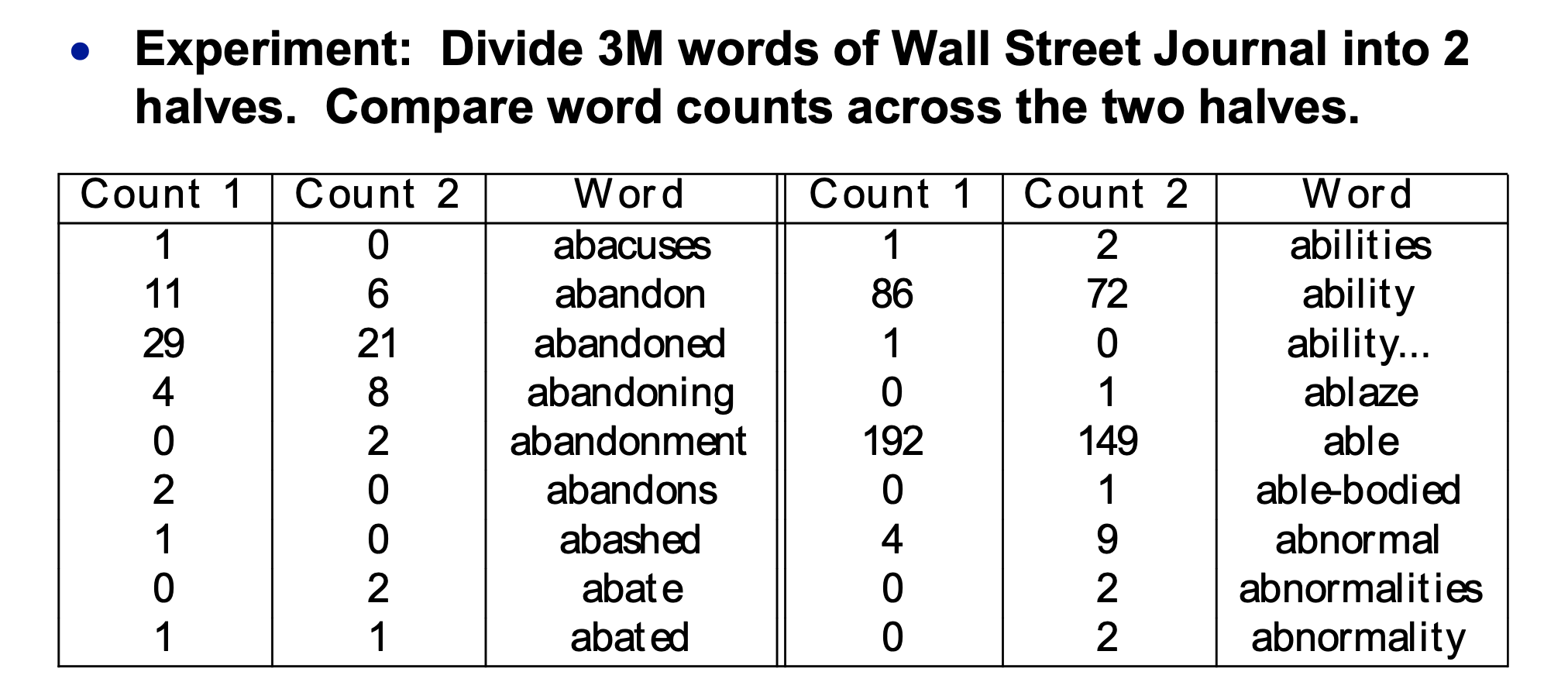
Let's empirically map out how much counts change between two samples of text from the same source. So we divide our training data into two halves 1 and 2. Here's the table of word counts:
 (from Mark Liberman
via Mitch Marcus)
(from Mark Liberman
via Mitch Marcus)
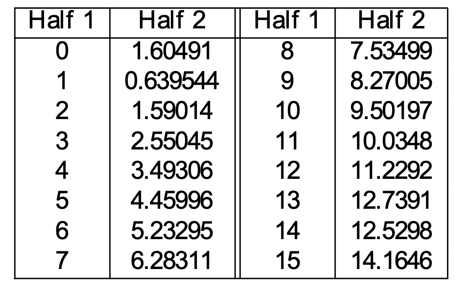
Now, let's pick a specific count r in the first half. Suppose that \(W_1,...,W_k\) are the words that occur r times in the first half. We can estimate the corrected count as
Corr(r) = average count of \(W_1,...,W_k\) in Half 2
This gives us the following correction table:
 (from Mark Liberman
via Mitch Marcus)
(from Mark Liberman
via Mitch Marcus)
Now, if there were \(n_1\) words in the first half of our data, we can use \(\text{Corr}(r)\over n_1\) as estimate of the true probability for each word \(W_i\) whose raw count was r.
Make the estimate symmetrical. Let's assume for simplicity that both halves contain the same number of words (at least approximately). Then compute
Corr(r) as above
Corr'(r) reversing the roles of the two datasets
\( {\text{Corr}(r) +\text{Corr}'(r)} \over 2\) estimate of the true count for a word with observed count r
Effectiveness of this depends on how we split the training data in half. Text tends to stay on one topic for a while. For example, if we see "boffin," it's likely that we'll see a repeat of that word soon afterwards. Therefore
These corrected estimates still have biases, but not as bad as the original ones. The method assumes that our eventual test data will be very similar to our training data, which is not always true.
Because training data is sparse, smoothing is a major component of any algorithm that uses n-grams. For single words, smoothing assigns the same probability to all unseen words. However, n-grams have internal structure which we can exploit to compute better estimates.
Example: how often do we see "cat" vs. "armadillo" on local subreddit? Yes, an armadillo has been seen in Urbana. But mentions of cats are much more common. So we would expect "the angry cat" to be much more common than "the angry armadillo". So
Idea 1: If we haven't seen an ngram, guess its probability from the probabilites of its prefix (e.g. "the angry") and the last word ("armadillo").
Certain contexts allow many words, e.g. "Give me the ...". Other contexts strongly determine what goes in them, e.g. "scrambled" is very often followed by "eggs".
Idea 2: Guess that an unseen word is more likely in contexts where we've seen many different words.
There's a number of specific ways to implement these ideas, largely beyond the scope of this course.