 Armadillo (picture from
Prairie Rivers Network)
Armadillo (picture from
Prairie Rivers Network)
The high level classification model is simple, but a lot of details are required to get high quality results. Over the next three videos, we'll look at four aspects of this problem:
Training data: estimate the probability values we need for Naive Bayes
Development data: tuning algorithm details
Test data: final evalution (not always available to developer) or the data seen only when system is deployed
Training data only contains a sampling of possible inputs, hopefully typically but nowhere near exhaustive. So development and test data will contain items that weren't in the training data. E.g. the training data might focus on apples where the development data has more discussion of oranges. Development data is used to make sure the system isn't too sensitive to these differences. The developer typically tests the algorithm both on the training data (where it should do well) and the development data. The final test is on the test data.
Results of classification experiments are often summarized into a few key numbers. There is often an implicit assumption that the problem is asymmetrical: one of the two classes (e.g. Spam) is the target class that we're trying to identify.
| Labels from Algorithm | ||
|---|---|---|
| Spam | Not Spam | |
| Correct = Spam | True Positive (TP) | False Negative (FN) |
| Correct = Not Spam | False Positive (FP) | True Negative (TN) |
We can summarize performance using the rates at which errors occur:
Or we can ask how well our output set contains all, and only, the desired items:
F1 is the harmonic mean of precision and recall. Both recall and precision need to be good to get a high F1 value.
For more details, see the Wikipedia page on recall and precision
We can also display a confusion matrix, showing how often each class is mislabelled as a different class. These usually appear when there are more than two class labels. They are most informative when there is some type of normalization, either in the original test data or in constructing the table. So in the table below, each row sums to 100. This makes it easy to see that the algorithm is producing label A more often than it should, and label C less often.
| Labels from Algorithm | |||
|---|---|---|---|
| A | B | C | |
| Correct = A | 95 | 0 | 5 |
| Correct = B | 15 | 83 | 2 |
| Correct = C | 18 | 22 | 60 |
We're now going to look at details required to make this classification algorithm work well.
Be aware that we're now talking about tweaks that might help for one application and hurt performance for another. "Your mileage may vary."
For a typical example of the picky detail involved in this data processing, see the method's section from the word cloud example in the previous lecture.
Our first job is to produce a clean string of words, suitable for use in the classifier. Suppose we're dealing with a language like English. Then we would need to
This process is called tokenization. Format features such as punctuation and capitalization may be helpful or harmful, depending on the task. E.g. it may be helpful to know that "Bird" is different from "bird," because the former might be a proper name. But perhaps we'd like to convert "Bird" to "CAP bird" to make its structure explicit. Similarly, "tyre" vs. "tire" might be a distraction or an important cue for distinguishing US from UK English. So "normalize" may either involve throwing away the information or converting it into a format that's easier to process.
After that, it often helps to normalize the form of each word using a process called stemming.
Stemming converts inflected forms of a word to a single standardized form. It removes prefixes and suffixes, leaving only the content part of the word (its "stem"). For example
       help, helping, helpful --->  help
       happy, happiness --> happi
Output is not always an actual word.
Stemmers are surprisingly old technology.
Porter made modest revisions to his stemmer over the years. But the version found in nltk (a currently popular natural language toolkit) is still very similar to the original 1980 algorithm.
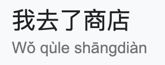
English has relatively short words, with convenient spaces between them. Tokenization requires slightly different steps for languages with longer words or different writing system. For example, Chinese writing does not put spaces between words. So "I went to the store" is written as a string of characters, each representing one syllable (below). So programs processing Chinese text typically run a "word segmenter" that groups adjacent characters (usually 2-3) into a word.
In German, we have the opposite problem: long words. So we might divide words like "Wintermantel" into "winter" (winter) and "mantel" (coat).
In either case, the output tokens should usually form coherent units, whose meaning cannot easily be predicted from smaller pieces.
Classification algorithms frequently ignore very frequent and very rare words. Very frequent words ("stop words") often convey very little information about the topic. So they are typically deleted before doing a bag of words analysis.
Rare words include words for uncommon concepts (e.g. armadillo), proper names, foreign words, and simple mistakes (e.g. "Computer Silence"). Words that occur only one often represent a large fraction (e.g. 30%) of the word types in a dataset. So rare words cause two problems
Rare words may be deleted. More often, all all rare words are mapped into a single placeholder value (e.g. UNK). This allows us to treat them all as a single item, with a reasonable probability of being observed.
The Bag of Words model uses individual words as features, ignoring the order in which they appeared. Text classification is often improved by using pairs of words (bigrams) as features. Some applications (notably speech recognition) use trigrams (triples of words) or even longer n-grams. E.g. "Tony the Tiger" conveys much more topic information than either "Tony" or "tiger". In the Boulis and Ostendorf study of gender classification bigram features proved significantly significantly more powerful.
For n words, there are \(n^2\) possible bigrams. But our amount of training data stays the same. So the training data is even less adequate for bigrams than it was for single words.