States are evaluated by a function f which estimates from start to goal via this state.
f(s) = g(s) + h(s)
g(s) is (actual) distance from the start state to s. h(s) is a heuristic estimate of the distance from s to the goal. f(s) is an estimate of the length of a path from start to goal via s.
Three types of states:
The frontier is stored in a priority queue, organized by the f values.
\(A^*\) finds the optimal path only when you do the bookkeeping correctly. The details are somewhat like UCS, but there are some new issues. Consider the following example (artificially cooked up for the purpoose of illustration).
(from Berkeley CS 188x materials)
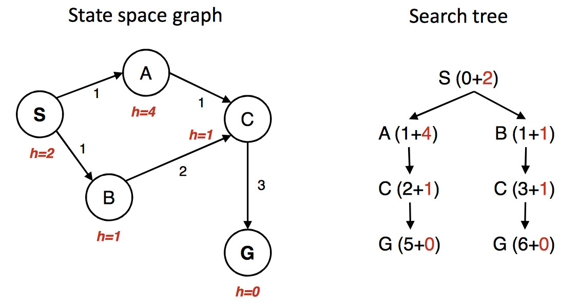
The state graph is shown on the left, with the h value under each state. The right shows a quick picture of the search process. Walking through the search in more detail:
First we put S in the queue with estimated cost 2, i.e. g(S) = 0 plus h(S) = 2.
We remove S from the queue and add its neighbors. A has estimated cost 5 and B has estimated cost 2. S is now done/closed.
We remove B from the queue and add its neighbor C. C has estimated cost 4. B is now done/closed.
We remove C from the queue. One of its neighbors (A) is already in the queue. So we only need to add G. G has cost 6. C is now done/closed.
We remove A from the queue. Its neighbors are all done, so we have nothing to do. A is now done.
We remove G from the queue. It's the goal, so we halt, reporting that the best path is SBCG with cost 6.
Oops. The best path is through A and has actual cost 5. But heuristic was admissible. What went wrong? Obviously we didn't do our bookkeeping correctly.
The algorithm we inherited from from UCS only updates costs for nodes that are in the frontier. In this example, paths through B look better at the start. So SBCG reaches C and G first. C and G are marked done/closed. And then we see the shorter path SAC. Updating the cost of C won't help because it's in the done/closed set.
Fix: when we update the cost of a node in the closed/done set, put that node back into the frontier (priority queue).
There is also a second issue, that applies also to UCS. Efficient priority queue implementations (e.g. the ones supplied with your favorite programming language) don't necessarily support updates to the priority numbers.
Workaround: it may be more efficient to put a second copy of the state (with the new cost) into the priority queue.
In many applications, decreases in state cost aren't very frequent. So this creates less inefficiency than using a priority queue implementation with more features.
The problem with shorter paths to old states is simplified if our heuristic is "consistent." That is, if we can get from n to n' with cost c(n,n'), we must have
\( h(s) \le c(s,s') + h(s') \)
So as we follow a path away from start state, our estimated cost f never decreases. Useful heuristics are often consistent. For example, the straight-line distance is consistent because of the triangle inequality.
When the heuristic is consistent, we never have to update the path length for a node that is in the done/closed set. (Though we may still have to update path lengths for nodes in the frontier.)
We can view UCS as A* with a heuristic function h that always returns zero. This heuristic is consistent, so updates to costs in UCS involve only states in the frontier.
There are many variants of A*, mostly hacks that may help for some problems and not others. See this set of pages for extensive implementation detail Amit Patel's notes on A*.
One well-known variant is iterative deepening A*. Remember that iterative deepening is based on a version of DFS ("length-bounded") in which search is stopped when the path reaches a target length k. Iterative deepening A* is similar, but search stops if the A* estimated cost f(s) is larger than k.
Another optimization involves building a "pattern database." This is a database of partial problems, together with the cost to solve the partial problem. The true solution cost for a search state must be at least as high as the cost for any pattern it contains.