|
|
CS440/ECE448 Fall 2021Assignment 6: Neural Nets and PyTorchDue date: Wednesday November 17th, 11:59pm |
The goal of this assignment is to employ neural networks, nonlinear and multi-layer extensions of the linear perceptron, to classify images into four categories: ship, automobile, dog, or frog. That is, your ultimate goal is to create a classifier that can tell what each picture depicts.
In the first part, you will create an 1980s-style shallow neural network. In the second part, you will improve this network using more modern techniques such as changing the activation function, changing the network architecture, or changing other initialization details.
You will be using the PyTorch and NumPy libraries to implement these models. The PyTorch library will do most of the heavy lifting for you, but it is still up to you to implement the right high-level instructions to train the model.
You will need to consult the PyTorch documentation, linked multiple times on this page, to help you with implementation details. We strongly recommend this PyTorch Tutorial since it walks you thorugh building a classifier very similar to the one in this assignment. There are also other guides out there such as this one.
The template package contains your starter code and also your training and development datasets (packed into a single file).
In the code package, you should see these files:
Modify only neuralnet_part1.py and neuralnet_part2.py.
Run python3 mp6.py -h in your terminal to find more about how to run the program.
There are gradaded two submit points on gradescope, and one optional submit point for entering your best network onto a leaderboard (which is ungraded). They are for part 1 (neuralnet_part1.py), part 2 (neuralnet_part2.py) and leaderboard (neuralnet_leaderboard.py,net.model and state_dict.state). The binary files net.model and param_dict.state are generated when you run mp6.py --part 3 and are used to load in your best model submission, whose architecture must be defined in neuralnet_leaderboard.pyb This will be the model used to give your score on the leaderboard. The leaderboard is sorted by your performance on the hidden test set, but this correlates well with the dev set performance. The leaderboard is only for bragging rights and is worth no points.
You will need to import torch and numpy. Otherwise, you should use only modules from the standard python library. Do not use torchvision .
A very recently released version of numpy (1.21.4) apparently has issues. Do not attempt to use it for this MP. Make sure you are using 1.21.3.
The autograder doesn't have a GPU, so it will fail if you attempt to use CUDA.
The dataset consists of 3000 32x32 colored (RGB) images (a subset of the CIFAR-10 dataset, provided by Alex Krizhevsky). This set is split for you into 2250 training examples (which are a mostly balanced sample of cars, boats, frogs and dogs) and 750 development examples.
The function load_dataset() in reader.py will unpack the dataset file, returning
images and labels for the training and development sets. Each of these items is
a Tensor.
Two of the inputs to your main training function (fit) are the number of epochs and the batch size. You should run your training process for that many epochs on the training set. In each epoch your code needs to process the data batch by batch, each batch having the specified size. If you try to do this by hand, you'll run into issues such as what to do when the dataset size isn't a multiple of the batch size.
To make this simple, you will use a pytorch dataloader.
A dataloader is a way for you to handle loading and transforming
data before it enters your network for training or prediction.
It will let you write code that looks like you're just looping through
the dataset, with the division into batches happening automatically.
Details on how to use a
dataloader can be found
in this
tutorial by Shervine Amidi. We have provided an auxiliary function
(get_dataset_from_arrays(X,Y)) in utils.py that converts tensors of
features (X) and labels (Y) into a simple torch dataset class that can
be loaded into their dataloaders for your convenience.
To get consistent output from the autograder, make sure to set "shuffle = False" on your dataloader.
The top-level program mp6.py returns three types of feedback about your model.
A confusion matrix is a very useful tool for evaluating multi-class classification problems, as it helps in identifying possible sources of imbalance in your dataset - and can offer precious insights into possible biases in your training procedure.
Specifically, in a classification problem with k classes, a confusion matrix will have k rows and k columns. Each row corresponds to the ground truth label of the data points - and each column refers to the predicted label by your classifier. Each entry on the matrix contains a count of the corresponding tuple (ground_truth label, predicted_label). In other words, all elements in the diagonal of this square matrix have been correctly classified - and all other elements count as mistakes. For instance, if your matrix has many entries in [0,1]. This will mean that your classifier tends to mistake points belonging to class 0 for points belonging to class 1. Further details can be found on this Wikipedia page.
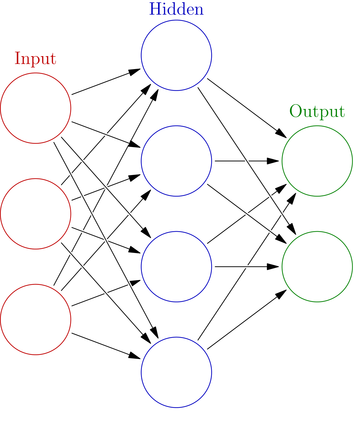
To make things more precise, in lecture you learned of a function \( f_{w}(x) = \sum_{i=1}^n w_i x_i + b\). In this assignment, given weight matrices \(W_1,W_2\) with \(W_1 \in \mathbb{R}^{h \times d}\), \(W_2 \in \mathbb{R}^{h \times 4}\) and bias vectors \(b_1 \in \mathbb{R}^{h}\) and \(b_2 \in \mathbb{R}^{4}\), you will learn a function \( F_{W} \) defined as \[ F_{W} (x) = W_2\sigma(W_1 x + b_1) + b_2 \] where \(\sigma\) is your activation function. In part 1, you should use either of the sigmoid or ReLU activation functions.
For this dataset, you have 3072 input values, one for each channel of each pixel in an image. That is \(d=(32)^2(3) = 3072\). You should be able to pass the Part 1 tests with no more than 200 hidden units. That is you should have \(h \le 200\).
Training: To train the neural network you are going to need to minimize the empirical risk \(\mathcal{R}(W)\) which is defined as the mean loss determined by some loss function. For this assignment you can use cross entropy for that loss function. In the case of binary classification, the empirical risk is given by \[ \mathcal{R}(W) = \frac{1}{n}\sum_{i=1}^n y_i \log \hat y_i + (1-y_i) \log (1 - \hat y_i) . \] where \(y_i\) are the labels and \(\hat y_i \) are determined by \(\hat y_i = \sigma(F_{W}(x_i))\) where \(\sigma(x) = \frac{1}{1+e^{-x}}\) is the sigmoid function. For this assignment, you won't have to implement these functions yourself; you can use the built-in PyTorch functions.
Notice that because PyTorch's CrossEntropyLoss incorporates a sigmoid function, you do not need to explicitly include an activation function in the last layer of your network.
Development: After you have trained your neural network model, you will have your model decide whether or not images in the development set decide what is the class of each image. This is done by evaluating your network \(F_{W}\) on each example in the development set, and then taking the index of the maximum of the four outputs (argmax).
Data Standardization: Convergence speed and accuracies can be improved greatly by simply centralizing your input data by subtracting the sample mean and dividing by the sample standard deviation. More precisely, you can alter your data matrix \(X\) by simply setting \(X:=(X-\mu)/\sigma\). Notice that you are standarizing a feature value across all images, not standardizing a feature value relative to the other features in the same image. This standardization should be done in the fit() function, not the forward() function.
Notice that the autograder will pass in the number of training epochs and the batch size. You don't control those. However, you do control the neural net's learning rate. If you are confident about a model you have implemented but are not able to pass the accuracy thresholds on gradescope, try increasing the learning rate. Be aware, however, that using a very high learning rate may worse performance since the model may begin to oscillate around the optimal parameter settings. With the above model design and tips, you should expect around 0.62 dev-set accuracy.
The files neuralnet_part1.py, neuralnet_part2.py and neuralnet_leaderboard.py give you a NeuralNet class which implements a torch.nn.module. This class consists of __init__(), forward(), and step() functions. The main function fit() will use these to train the network and then classify the images from the test/development set.
__init__() __init__() is where you will need to construct the network architecture.
There's two ways to do this:
Linear and Sequential objects.
Keep in mind that Linear uses a Kaiming He uniform initialization to initialize the weight
matrices and sets the bias terms to all zeros.Tensors. This
approach is more hands on and will allow you to choose your
own initialization. For this assignment, however, Kaiming He
uniform initialization should suffice and should be a good
choice.Look at the examples in the PyTorch Tutorial.
forward()forward() should perform a forward pass through your network. This means
it should explicitly evaluate \(F_{W}(x)\) . This can be done by simply calling your Sequential
object defined in __init__() or (if you opted to define tensors explicitly) by multiplying through the weight
matrices with your data.
step()step() should perform
the gradient update through one batch of training data (not the entire set of training
data). You can do this by either calling loss_fn(yhat,y).backward()
then updating the weights directly yourself, or you can use an optimizer object that you
may have initialized in __init__() to help you update the network.
Be sure to call zero_grad()
on your optimizer in order to clear the gradient buffer.
When you return the loss_value from this function, make sure to convert it to a plain number. This allows proper garbage collection to take place, so that your program won't consume excessive amounts of memory. Two options:
loss_value.item(). This works if it is just a single number.
loss_value.detach().cpu().numpy(). This which
separates the loss value from the computations that led up to it,
moves it to the CPU (e.g. if you are using a GPU locally), and
then converts it to a NumPy array.
Remember that Gradescope won't have a GPU.
fit()fit() should construct a NeuralNet object,
and iteratively call the neural net's step() function to train the network.
The inputs to fit() tell you the batch size and how many training epochs you should use.
fit() should then run the neural net on the development set and
return 3 things: a list of the losses for each epoch of training, a numpy array with the estimated class labels (0, 1, 2, or 3) for the dev set and the trained network.
In this part, you will try to improve your performance by employing modern machine learning techniques. These include, but are not limited to, the following:
Try to make your classification accuracy as high as possible, subject to the constraint that you may use at most 500,000 total parameters. This means that if you take every floating point value in all of your weights including bias terms, i.e. as returned by this pytorch utility function, you only use at most 500,000 floating point values.
You should be able to get an accuracy of at least 0.79 on the development set.
If you're using a convolutional net, you need to reshape your data in
the forward() method, and not the fit() method. The autograder will
call your forward function on data with shape (N,3072).
That's probably not what your CNN is expecting. It's helpful to print out the
shape of key objects when trying to debug dimension issues. (the .view() method from tensors is very useful here)
Apparently it's still possible to be using a 32-bit environment. This may be ok. However, be aware that recent versions of PyTorch are optimized for a 64-bit environment and that is what Gradescope is using.
For your own enjoyment, we have provided also an anonymous leaderboard for this MP. Even after you have full points on Part 2, you may wish to try even more things to improve your performance on the hidden test set by tuning your network better, training it for longer, using dropouts, data augmentations, etc. For the leaderboard, you can submit the net.model and state_dict.state created with your best trained model (after running mp6.py --part 3) alongside neuralnet_leaderboard.py (note that these need not implement the same thing, as you could wish to do fancy things that would be too slow for the autograder). We will not train this specific network on the autograder, so if you wish to go wild with augmentations, costly transformations, more complex architectures, you're welcome to do so. Just do not exceed the 500k parameter limit, or your entry will be invalid. Also, please do not use additional external data for the sake of fairness (i.e. using a resnet backbone trained on ImageNet would be very unfair and counterproductive).