| CS440/ECE448 Fall 2020Assignment 6: Neural Nets and PyTorchDue date: Wednesday November 18th, 11:55pm |
Created By: Justin Lizama, Kedan Li, and Tiantian Fang
Updated Fall 2020: Jatin Arora, Kedan Li, and Michal Shlapentokh-Rothman
The goal of this assignment is to extend your results from MP5, improving the accuracy by employing neural networks (also known as multilayer perceptrons), nonlinear extensions of the linear perceptron from MP5. In the first part, you will create an 1980s style shallow neural network. In the second part, the goal is to improve this network using more modern techniques such as changing the activation function and/or changing the network architecture or initialization details.
You will be using the PyTorch and NumPy library to implement these models. The PyTorch library will do most of the heavy lifting for you, but it is still up to you to implement the right high level instructions to train the model.
Contents
- Dataset
- Part 1: Classical Shallow Networks
- Part 2: Modern Networks
- Provided Code Skeleton
- Deliverables
Dataset
The dataset consists of 10000 32x32 colored images total. We have split this data set for you into 2500 development examples and 7500 training examples. There are 2999 negative examples and 4501 positive examples in the training set. This is a subset of the CIFAR-10 dataset, provided by Alex Krizhevsky.
The data set can be downloaded here:
data (gzip) or
data (zip). When you uncompress this you'll find
a binary object that our reader code will unpack for you.
To make things more precise, in MP5 you learned a function \( f_{w}(x) = \sum_{i=1}^n w_i x_i + b\).
In this assignment, given weight matrices \(W_1,W_2\) with \(W_1 \in \mathbb{R}^{h \times d}\), \(W_2 \in \mathbb{R}^{h \times 2}\)
and bias vectors \(b_1 \in \mathbb{R}^{h}\) and \(b_2 \in \mathbb{R}^{2}\), you will
learn a function \( F_{W} \) defined:
\[
F_{W} (x) = W_2\sigma(W_1 x + b_1) + b_2
\]
where \(\sigma\) is your activation function. In part 1, you should use either
sigmoid or ReLU activation functions.
You will use
32 hidden units (\(h=32\)) and 3072 input units, one for each of the image's pixels
(\(d=(32)(32)(3) = 3072\)).
Notice that torch.nn.CrossEntropyLoss() incorporates a sigmoid function.
So you do not need to explicitly include an activation function in the last layer
of your network.
We have provided
( tar
zip)
all the code to get you started on your MP, which
means you will only have to implement PyTorch neural network model.
In the __init__() function you will need to construct the network architecture.
There are multiple ways to do this. One way is to use nn.Linear() and nn.Sequential() .
Keep in mind that nn.Linear() uses a Kaiming He uniform initialization to initialize the weight matrices and 0 for
the bias terms. Another way you could do things is by explicitly defining weight matrices W1,W2,... and bias
terms b1,b2,... by defining them as a torch.tensor(). This way is more hands on and will allow you to choose
your own initialization. However, for this assignment Kaiming He uniform initialization should suffice and should be a good choice.
Additionally, you can initialize a torch.optim optimizer object in this function to use
to optimize your network in the step() function.
The forward() function should do a forward pass through your network. This means
it should explicitly evaluate \(F_{W}(x)\) . This can be done by simply calling your nn.Sequential()
object defined in __init__() or in the torch.tensor() case by explicitly multiplying the weight matrices by your data.
The step() function should perform one iteration of training. This means it should
perform one gradient update through one batch of training data (not the entire set of training data). You can do this by calling loss_fn(yhat,y).backward()
then either update the weights directly yourself, or you can use a torch.optim object that you
may have initialized in __init__() to help you update the network. Be sure to call zero_grad()
on your optimizer in order to clear the gradient buffer. When you return the loss value from this function, make sure
you return loss_value.item() (works only if its just a single number)
or loss_value.detach().cpu().numpy(). This makes sure that the returned loss value is detached from the computational graph
after one execution of the step() function and proper garbage collection can take place (else your program might
exceed the memory limits fixed on gradescope).
More details on what each of these methods in the NeuralNet class should do is given in
the skeleton code.
The function fit() takes as input the training data, training labels, development set, and maximum number of
iterations. The training data provided is the output from reader.py.
The training labels is a torch tensor consisting of labels corresponding to each image in the training data.
The development set is the torch tensor of images that you are going to test your implementation on.
The maximium number of iterations is the number you specified with --max_iter (it is 500 by default).
fit() outputs the predicted labels.
The fit function should construct a NeuralNet object,
and iteratively call the neural net's step() function to train the network. This should be
done by feeding in batches of data determined by batch size. You will use a batch size of 100 for this assignment. max_iter is the number of batches (not the number of epochs) in your training process.
Do not modify the provided code. You will only have to modify neuralnet_part1.py and neuralnet_part2.py.
To understand more about how to run the MP, run python3 mp6.py -h in your terminal.
Definitely use the PyTorch docs to help you with implementation details.
You can also use this PyTorch Tutorial as a reference to help you
with your implementation. There are also other guides out there such as this one.
This MP will be submitted via gradescope. There are 2 submission points corresponding to the 2 parts in the assignment statement.
Please upload neuralnet_part1.py (for part1) and neuralnet_part2.py (for part 2) to gradescope.Part 1: Classical Shallow Network
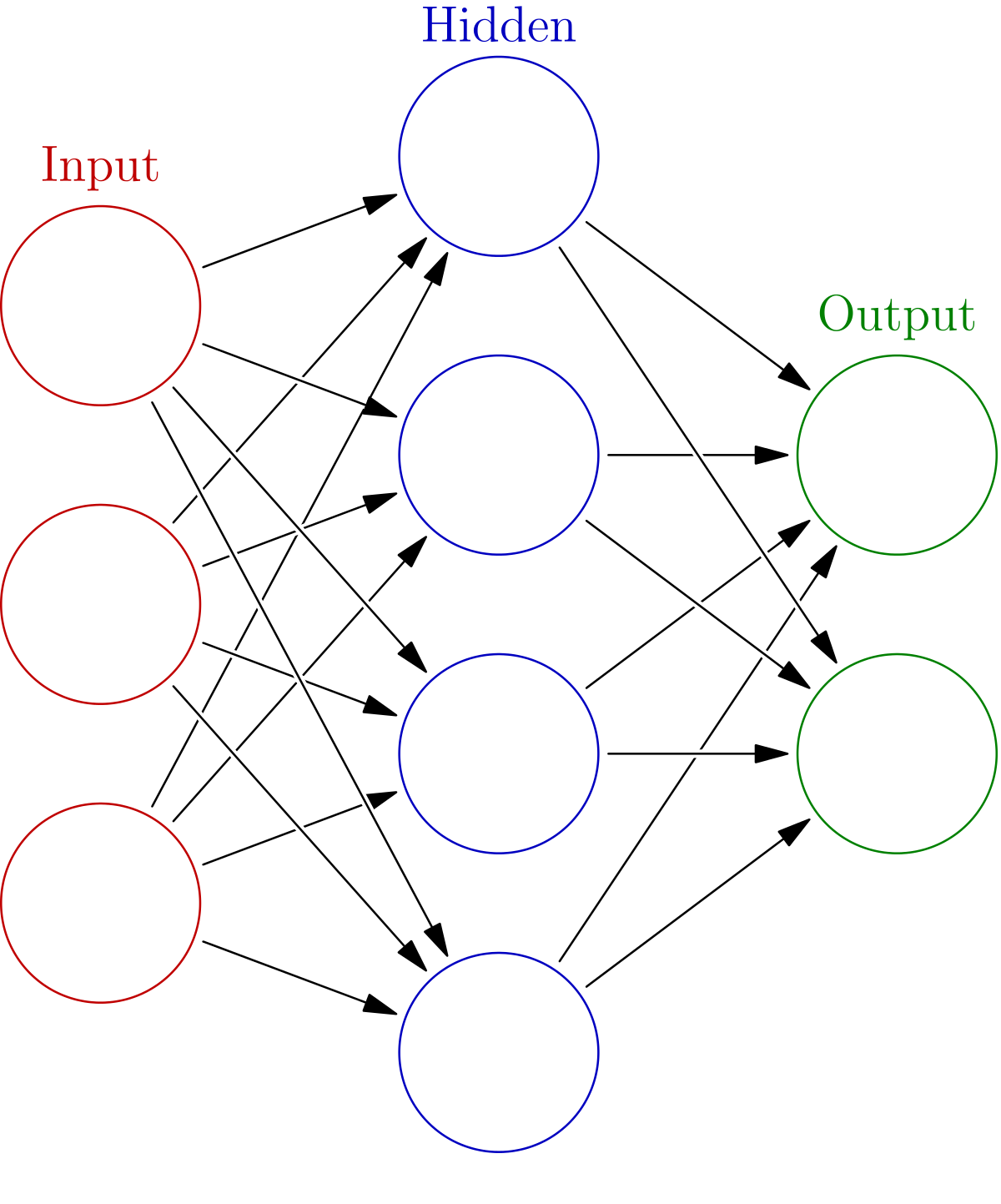
The basic neural network model consists of a sequence of hidden layers
sandwiched by an input and output layer. Input is fed into it from the
input layer and the data is passed through the hidden layers and out to the output layer.
Induced by every neural network is a function \(F_{W}\) which is given by propagating the data
through the layers.
Training and Development
With the above mentioned model design and tips, you should expect dev-set accuracy around
0.84.
Part 2: Modern Network
In this part, you will try to improve your performance by employing more modern machine learning techniques.
These include, but are not limited to the following:
Try to employ some of these techniques in order to attain a dev-set accuracy around
0.87. The only stipulation is that you use under 500,000 total parameters. This means
that if you take every floating point value in all of your weights including bias terms, you only use
at most 500,000 floating point values.
Some things to look for:
Provided Code Skeleton
Updated Code Files (11/10/2020, Tuesday, 1AM CT): We have updated reader.py
(added a new function to set seeds for random initializations done by PyTorch) and mp6.py
(called the init_seeds function at the top of main function). This is just to help you get the same consistent
behavior on dev set in your local and gradescope (no changes in logic or anything else).
Deliverables