| CS440/ECE448 Fall 2019Assignment 6: Neural Nets and PyTorchDue date: Monday November 18th, 11:55pm |
Created By: Justin Lizama, Kedan Li, and Tiantian Fang
The goal of this assignment is to extend your results from MP5, improving the accuracy by employing neural networks (also known as multilayer perceptrons), nonlinear extensions of the linear perceptron from MP5. In the first part, you will create an 1980s style neural network with sigmoid activation functions. In the second part, the goal is to improve this network using more modern techniques such as changing the activation function and/or changing the network architecture or initialization details.
You will be using the PyTorch and NumPy library to implement these models. The PyTorch library will do most of the heavy lifting for you, but it is still up to you to implement the right high level instructions to train the model.
Contents
- Dataset
- Part 1: Classical Sigmoid Networks
- Part 2: Modern Networks
- Extra Credit Suggestion
- Provided Code Skeleton
- Deliverables
Extra credit may be awarded for going beyond expectations or
completing the suggestions below. Notice, however, that the score for
each MP is capped at 110%.
The dataset consists of 10000 32x32 colored images total. We have
split this data set for you into 2500 development examples and 7500 training
examples. There are 2999 negative examples and 4501 positive examples in the
training set.
This is a subset of the CIFAR-10 dataset,
provided by Alex Krizhevsky.
The data set can be downloaded here:
data (gzip) or
data (zip). When you uncompress this you'll find
a binary object that our reader code will unpack for you.
To make things more precise, in MP5 you learned a function \( f_{w}(x) = \sum_{i=1}^n w_i x_i + b\).
In this assignment, given weight matrices \(W_1,W_2\) with \(W_1 \in \mathbb{R}^{h \times d}\), \(W_2 \in \mathbb{R}^{2 \times h}\)
and bias vectors \(b_1 \in \mathbb{R}^{h}\) and \(b_2 \in \mathbb{R}^{2}\), you will
learn a function \( F_{W} \) defined:
\[
F_{W} (x) = W_2\sigma(W_1 x + b_1) + b_2
\]
where \(\sigma\) is your activation function. In part 1, we will be using the sigmoid
activation function which is defined \(\sigma(x) = \frac{1}{1+e^{-x}}\), and
we will have \(h=32\) and \(d=(32)(32)(3) = 3072\). In other words, we will be using
32 hidden units and we will have 3072 input units, one for each of the image's pixels.
While it is possible to obtain nice results with traditional multilayer perceptrons,
when doing image classification tasks it is often best to use convolutional neural
networks, which are tailored specifically to signal processing tasks such as
image recognition. See if you can improve your results using convolutional
layers in your network.
Additionally, there are several other techniques besides L2 regularization
for improving the generalization of your model. Some ideas are dropout, batch normalization, and
choice of loss function. You could also see how far you can take these
regularization methods to improve your model.
There will be a leaderboard ranking the best models. However, all you need to do
to get the full extra credit points is to attain an accuracy of at least 88%.
We have provided
( tar
zip)
all the code to get you started on your MP, which
means you will only have to implement PyTorch neural network model.
In the __init__() function you will need to construct the network architecture.
There are multiple ways to do this. One way is to use nn.Linear() and nn.Sequential() .
Keep in mind that nn.Linear() uses a Kaiming He uniform initialization to initialize the weight matrices and 0 for
the bias terms. Another way you could do things is by explicitly defining weight matrices W1,W2,... and bias
terms b1,b2,... by defining them as a torch.tensor(). This way is more hands on and will allow you to choose
your own initialization. However, for this assignment Kaiming He uniform initialization should suffice and should be a good choice.
Additionally, you can initialize a torch.optim optimizer object in this function to use
to optimize your network in the step() function.
The forward() function should do a forward pass through your network. This means
it should explicitly evaluate \(F_{W}(x)\) . This can be done by simply calling your nn.Sequential()
object defined in __init__() or in the torch.tensor() case by explicitly multiplying the weight matrices by your data.
The step() function should perform one iteration of training. This means it should
perform one gradient update through your training data. You can do this by calling loss_fn(yhat,y).backward()
then either update the weights directly yourself, or you can use a torch.optim object that you
may have initialized in __init__() to help you update the network. Be sure to call zero_grad()
on your optimizer in order to clear the gradient buffer.
More details on what each of these methods in the NeuralNet class should do is given in
the skeleton code.
The function fit() takes as input the training data, training labels, development set, and maximum number of iterations. The training data provided is the output from reader.py.
The training labels is a torch tensor consisting of labels corresponding to each image in the training data.
The development set is the torch tensor of images that you are going to test your implementation on.
The maximium number of iterations is the number you specified with --max_iter (it is 10 by default).
fit() outputs the predicted labels. The fit function should construct a NeuralNet object,
and iteratively call the neural net's step() function to train the network. This should be
done by feeding in batches of data determined by batch size. (You will use a batch size of 100 for this assignment.)
Do not modify the provided code. You will only have to modify neuralnet.py.
To understand more about how to run the MP, run python3 mp6.py -h in your terminal.
Definitely use the PyTorch docs to help you with implementation details.
You can also use this PyTorch Tutorial as a reference to help you
with your implementation. There are also other guides out there such as this one.
This MP will be submitted via gradescope.
When you believe your model has attained an acceptable accuracy on the development set,
save your trained model by using the torch.save() function. You should save your model
in a file named net.model, and submit it together with your neuralnet.py
Please upload only neuralnet.py and net.model to gradescope.Dataset
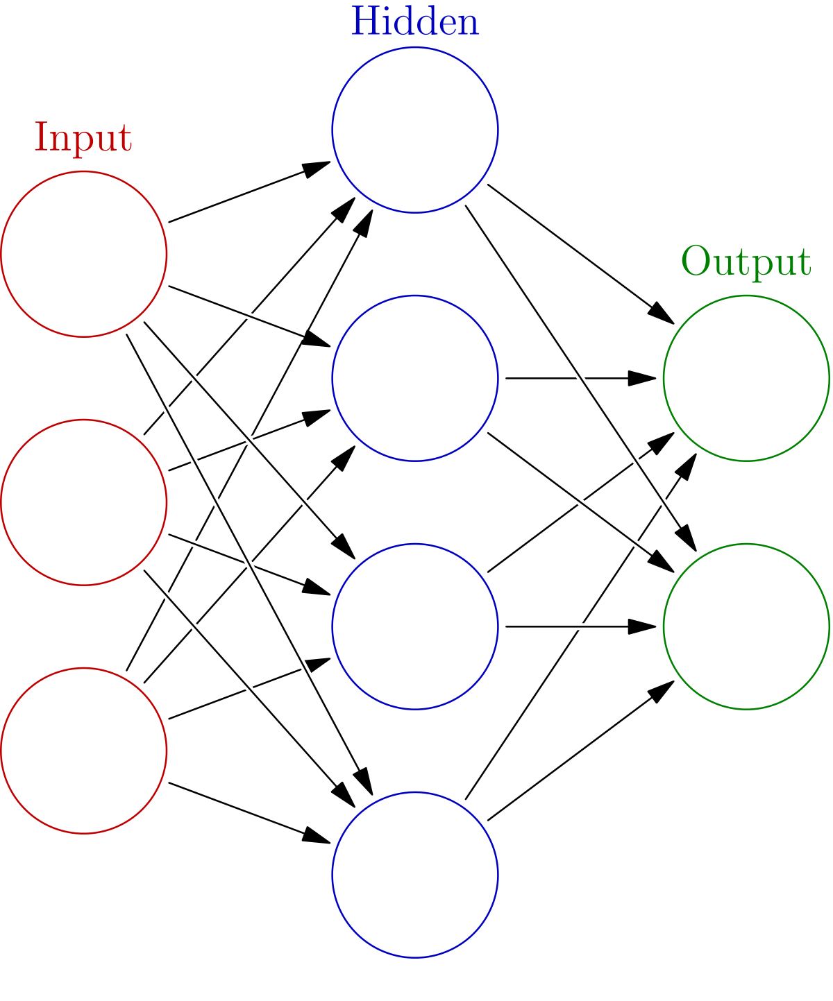
Part 1: Classical Sigmoid Network
The basic neural network model consists of a sequence of hidden layers
sandwiched by an input and output layer. Input is fed into it from the
input layer and the data is passed through the hidden layers and out to the output layer.
Induced by every neural network is a function \(F_{W}\) which is given by propagating the data
through the layers.
Training and Development
Part 2: Modern Network
In this part, you will try to improve your performance by employing more modern machine learning techniques.
These include, but are not limited to the following:
Try to employ some of these techniques in order to attain a test accuracy of at least
0.84. The only stipulation is that you use under 500,000 total parameters. This means
that if you take every floating point value in all of your weights including bias terms, you only use
at most 500,000 floating point values.
Extra Credit Suggestion
Provided Code Skeleton
Deliverables