We'd like to convert the context of a word w (aka words seen near w) to short, informative feature vectors. Previous methods did this in two steps:
Last lecture, we saw two methods of normalization: TF-IDF and PMI.
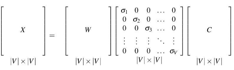
Both TF-IDF and PMI methods create vectors that contain informative numbers but still very long and sparse. For most applications, we would like to reduce these to short dense vectors that capture the most important dimensions of variation. A traditional method of doing this uses the singular value decomposition (SVD).
Theorem: any rectangular matrix can be decomposed into three matrices:
 from Dan Jurafsky at Stanford.
In the new coordinate system (the input/output of the S matrix), the information in our original vectors is represented by a set of orthogonal vectors. The values in the S matrix tell you how important each basis vector is, for representing the data. We can make it so that weights in S are in decreasing order top to bottom.
It is well-known how to compute this decomposition. See a scientific computing text for methods to do it accurately and fast. Or, much better, get a standard statistics or numerical analysis package to do the work for you.
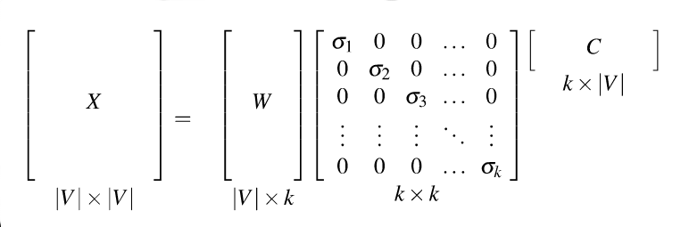
Recall that our goal was to create shorter vectors. The most important information lies in the top-left part of the S matrix, where the S values are high. So let's consider only the top k dimensions from our new coordinate system: The matrix W tells us how to map our input sparse feature vectors into these k-dimensional dense feature vectors.
 from Dan Jurafsky at Stanford.
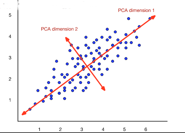
The new dimensions are called the "principal components." So this technique is often called a principal component analysis (PCA). When this approach is applied to analysis of document topics, it is often called "latent semantic analysis" (LSA).
 from Dan Jurafsky at Stanford.
Bottom line on SVD/PCA
The word2vec (aka skip-gram) algorithm is a newer algorithm that does normalization and dimensionality reduction in one step. That is, it learns how to embed words into an n-dimensional feature space. The algorithm was introduced in a couple papers by Mikolov et al in 2013. However, it's pretty much impossible to understand the algorithm from those papers, so the following derivation is from later papers by Yoav Goldberg and Omer Levy. (See paper references at the end of this web page.)
In broad outline word2vec has three steps
A pair (w,c) is considered "similar" if the dot product \(w\cdot c\) is large.
For example, our initial random embedding might put "elephant" near "matchbox" and far from "rhino." Our iterative adjustment would gradually move the embedding for "rhino" nearer to the embedding for "elephant."
Two obvious parameters to select. The dimension of the embedding space would depend on how detailed a representation the end user wants. The size of the context window would be tuned for good performance.
Problem: a great solution for the above optimization problem is to map all words to the same embedding vector. That defeats the purpose of having word embeddings.
Suppose we had negative examples (w,c'), in which c' is not a likely context word for w. Then we could make the optimization move w and c' away from each other. Revised problem: our data doesn't provide negative examples.
Solution: Train against random noise, i.e. randomly generate "bad" context words for each focus word.
The negative training data will be corrupted by containing some good examples, but this corruption should be a small percentage of the negative training data.
Another mathematical problem happens when we consider a word w with itself as context. The dot product \(w \cdot w\) ls large, by definition. But, for most words, w is not a common context for itself, e.g. "dog dog" is not very common compared to "dog." So setting up the optimization process in the obvious way causes the algorithm to want to move w away from itself, which it obviously cannot do.
To avoid this degeneracy, word2vec builds two embeddings of each word w, one for w seen as a focus word and one for w used as a context word. The two embeddings are closely connected, but not identical. The final representation for w will be a concatenation of the two embedding vectors.
Our classifier tries to predict yes/no from pairs (w,c), where "yes" means c is a good context word for w.
We'd like to make this into a probabilistic model. So we run dot product through a sigmoid to produce a "probability" that (w,c) is a good word-context pair. These numbers probably aren't the actual probabilities, but we're about to treat them as if they are. That is, we approximate
\( P(\text{good} | w,c) \approx \sigma(w\cdot c). \)
By the magic of exponentials (see below), this means that the probability that (w,c) is not a good word-context pair is
\( P(\text{bad} | w,c) \approx \sigma(-w\cdot c). \)
Now we switch to log probabilities, so we can use addition rather than multiplication. So we'll be looking at e.g.
\(\log( P(\text{good} | w,c)) \approx \log(\sigma(w\cdot c)) \)
Suppose that D is the positive training pairs and D' is the set of negative training pairs. So our iterative refinement algorithm adjusts the embeddings (both context and word) so as to maximize
\( \sum_{(w,c) in D} \ \log(\sigma(w\cdot c)) + \sum_{(w,c) in D'} \ \log(\sigma(-w\cdot c)) \)
That is, each time we read a new focus word w from the training data, we
Ok, so how did we get from \( P(\text{good} | w,c) = \sigma(w\cdot c) \) to \( P(\text{bad} | w,c) = \sigma(-w\cdot c) \)?
"Good" and "bad" are supposed to be opposites. So \( P(\text{bad} | w,c) = \sigma(-w\cdot c) \) should be equal to \(1 - P(\text{good}| w,c) = 1- \sigma(w\cdot c) \). I claim that \(1 - \sigma(w\cdot c) = \sigma(-w\cdot c) \).
This claim actually has nothing to do with the dot products. As a general thing \(1 - \sigma(x) = \sigma(-x) \). Here's the math.
Recall the definition of the sigmoid function: \( \sigma(x) = \frac{1}{1+e^{-x}} \).
\( \eqalign{ 1-\sigma(x) &=& 1 - \frac{1}{1+e^{-x}} = \frac{e^{-x}}{1+ e^{-x}} \ \ \text{ (add the fractions)} \\ &=& \frac{1}{1/e^{-x}+ 1} \ \ (\text{divide top and bottom by } e^{-x}) \\ &=& \frac{1}{e^x + 1} \ \ \text{(what does a negative exponent mean?)} \\ &=& \frac{1}{1 + e^x} = \sigma(-x)} \)
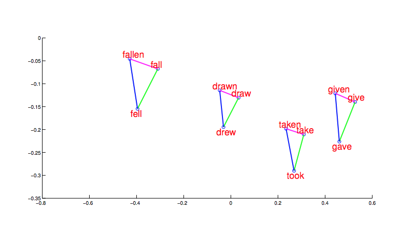
Even the final word embeddings still involve vectors that are too long to display conveniently. Projections onto two dimensions (or three dimensions with moving videos) are hard to evaluate. More convincing evidence for the coherency of the output comes from word relationships. First, notice that morphologically related words end up clustered. And, more interesting, the shape and position of the clusters are the same for different stems.
 from Mikolov,
NIPS 2014
from Mikolov,
NIPS 2014
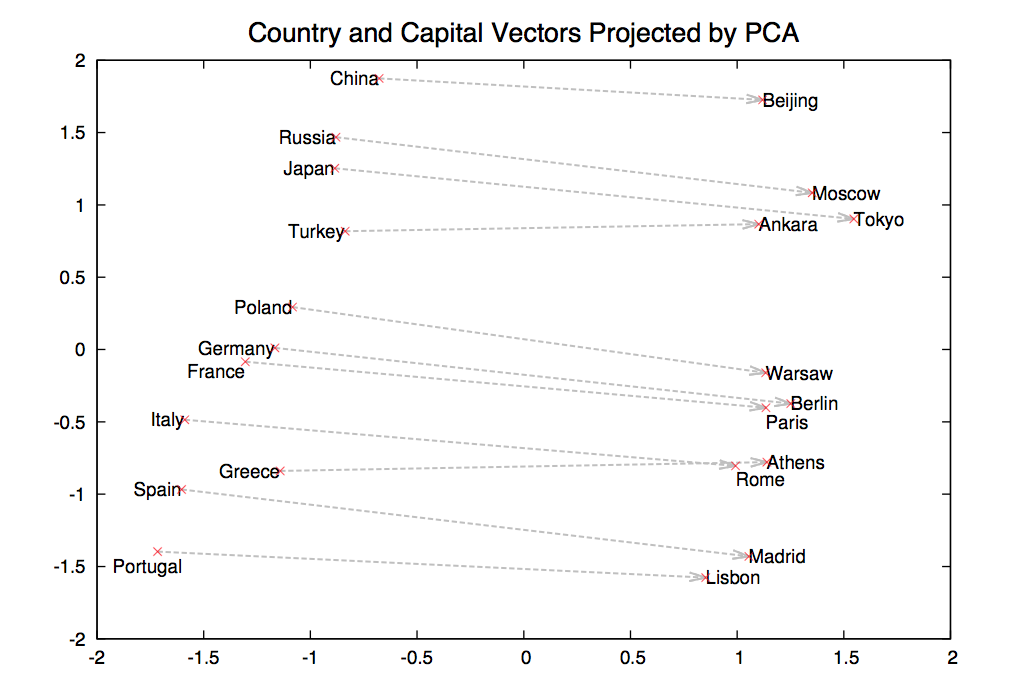
Now suppose we find a bunch of pairs of words illustrating a common relation, e.g. countries and their capitals in the figure below. The vectors relating the first word (country) to the second word (capital) all go roughly in the same direction.
 from Mikolov,
NIPS 2014
from Mikolov,
NIPS 2014
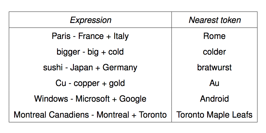
We can get the meaning of a short phrase by adding up the vectors for the words it contains. But we can also do simple analogical reasoning by vector addition and subtraction. So if we add up
vector("Paris") - vector("France") + vector("Italy")
We should get the answer to the analogy question "Paris is to France as ?? is to Italy". The table below shows examples where this calculation produced an embedding vector close to the right answer:
 from Mikolov,
NIPS 2014
from Mikolov,
NIPS 2014
Two similar embedding algorithms (which we won't cover) are the CBOW algorithm from word2vec and the GloVe algorithm from Stanford.
Original Mikolov et all papers:
Goldberg and Levy papers (easier and more explicit)