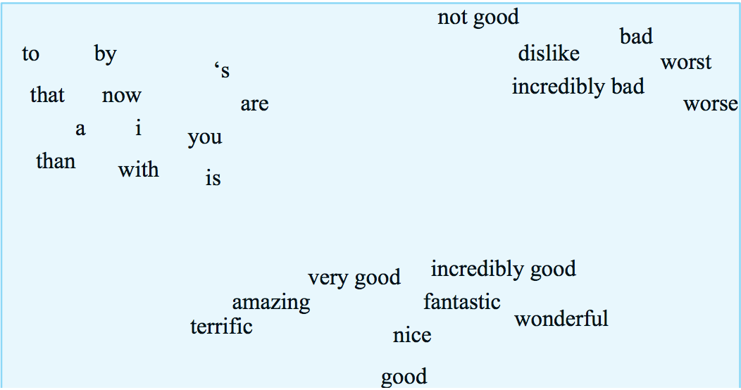
We're hoping to map ("embed") each word into a position in a vector space with a modest number of dimensions (e.g. 100) such that similar words are near one another. Ideally so it looks clean and reasonable as in the picture below. Our measures of similarity will be based on what words occur near one another in a text data corpus, because that's the type of data that's available in quantity.
 from Jurafsky and Martin
Feature vectors are based on some context that the focus word occurs in. There are a continuum of possible contexts, which will give us different information:
Close neighbors tend to tell you about the word's syntactic properties (e.g. part of speech. Nearby words tend to tell you about it's main meaning. The document tends to tell you what topic it comes from (e.g. math letures vs. Harry Potter).
For example, we might count how often each word occurs in each of a group of documents, e.g. the following table of selected words that occur in various plays by Shakespeare. These counts give each word a vector of numbers, one per document.
| As You Like It | Twelfth Night | Julius Caesar | Henry V | |
|---|---|---|---|---|
| battle | 1 | 0 | 7 | 13 |
| good | 114 | 80 | 62 | 89 |
| food | 36 | 58 | 1 | 4 |
| wit | 20 | 15 | 2 | 3 |
We can also used these word-document matrices to produce a feature vector for each document, describing its topic. These vectors would typically be very long (e.g. one value for every word that is used in any of the documents). This representation is primarily used in document retrieval, which is historically the application for which many vector methods were developed.
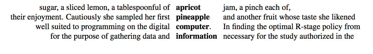
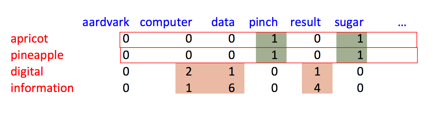
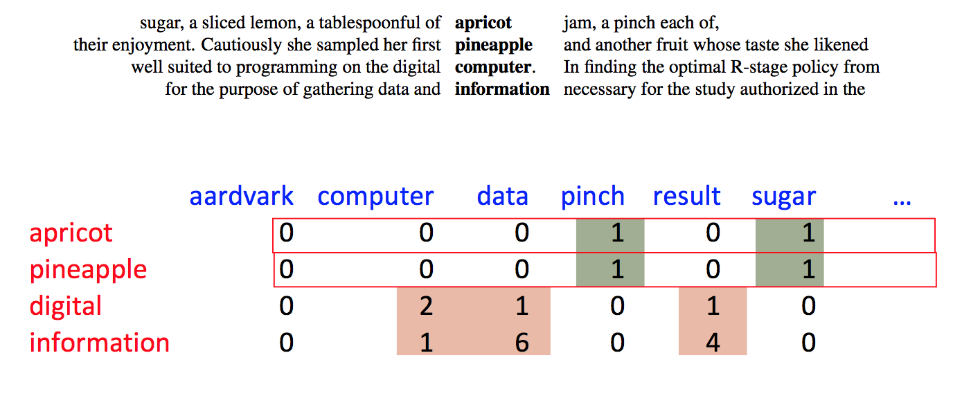
Alternative, we can use nearby words as context. So this example from Jurafsky and Martin shows sets of 7 context words to each side of the focus word. Our 2D data table will relate each focus word to each context word.
These features don't (even after appropriate massaging) provide a complete model of word meanings. However, as we've seen earlier with neural nets, they provide representations that are good enough to work well in many practical tasks.
Suppose we have a vector of word counts for each document. How do we measure similarity between documents?
Notice that short documents have fewer words than longer ones. So we normally consider only the direction of these feature vectors, not their lengths. So we actually want to compare the directions of these vectors. The smaller the angle between them, the more similar they are.
(2, 1, 0, 4, ...)
(6, 3, 0, 8, ...) same as previous
(2, 3, 1, 2, ...) different
This analysis applies also to feature vectors for words: rare words have fewer observations than common ones.
The actual angle is hard to work with, e.g. we can't compute it without calling an inverse trig function. It's much easier to approximate the angle with its cosine.
Recall what the cosine function looks like
What happens past 90 degrees? Oh, word counts can't be negative! So our vectors all live in the first quadrant, so their angles can't differ by more than 90 degrees.
Recall a handy formula for computing the cosine of the angle \(\theta\) between two vectors:
input vectors \(v = (v_1,v_2,\ldots,v_n) \) and \(w = (w_1,w_2,\ldots,w_n) \)
dot product: \( v\cdot w = v_1w_1 + ... + v_nw_n\)
\( \cos(\theta) = \frac{v \cdot w}{|v||w|} \)
So you'll see both "cosine" and "dot product" used to describe this measure of similarity.
Raw word count vectors don't work very well. There are two basic issues:
We'll first see older methods in which these two steps are distinct. Word2vec (next lecture) accomplishes both via one procedure.
Why don't raw word counts work well?
In terms of the item we're trying to classify
In terms of the words/documents we're using as context
TF-IDF normalization maps word counts into a better measure of their importance for classification. It is a bit of a hack, but one that has proved very useful in document retrieval. To match the historical development, suppose we're trying to model the topic of a document based on counts of how often each word occurs in it.
Suppose that we are looking at a particular focus word in a particular focus document. The TF-IDF feature is the product of TF (normalized word count) and IDF (inverse document frequency).
Warning: neither TF nor IDF has a standard definition, and the most common definitions don't match what you might guess from the names. Here is one of many variations on how to define them.
To keep things simple, let's assume that our word occurs at least once. It's pretty much universal that smoothing methods leave 0 counts unchanged.
To compute TF, we smooth the raw count c for the word. \(\log{c}\) is a better measure of the importance of the word. Many studies of humans suggest that our perceptions are well modelled by a log scale. Also, the log transformation reduces the impact of correlations (repeated words) within a document. However, \(\log{c}\) maps 1 to zero and exaggerates the importance of very rare words. So it's more typical to use
TF = \(1+\log_{10}(c)\)
The document frequency (DF) of the word, is df/N, where N is the total number of documents and df is the number our word appears in. When DF is small, our word provides a lot of information about the topic. When DF is large, our word is used in a lot of different contexts and so provides little information about the topic.
The normalizing factor IDF is also typically put through a log transformation, for the same reason that we did this to TF:
IDF = \( \log_{10}(N/df)\)
To avoid exaggerating the importance of very small values of N/df, it's typically better to use this:
IDF = \( \log_{10}(1+ N/df)\)
The final number that goes into our vector representation is TF*IDF. That is, we multiply the two quantities even though we've already put them both onto a log scale. I did say this was a bit of a hack, didn't I?
Let's switch to our other example of feature vectors: modelling a word's meaning on the basis of words seen near it in running text. We still have the same kinds of normalization/smoothing issues.
Here's a different (but also long-standing) approach to normalization. We've picked a focus word w and a context word c. We'd like to know how closely our two words are connected. That is, do they occur together more often than one might expect for independent draws?
Suppose that w occurs with probability P(w) and c with probability P(c). If the two were appearing independently in the text, the probability of seeing them together would be P(w)P(c). Our actual observed probability is P(w,c). So we can use the following fraction to gauge how far away they are from independent:
\( \frac {P(w,c)}{P(w)P(c)} \)
Example: consider "of the" and "three-toed sloth." The former occurs a lot more often. However, that's mostly because its two constituent words are both very frequent. The PMI normalizes by the frequencies of the constituent words.
Putting this on a log scale gives us the pointwise mutual information (PMI)
\( I(w,c) = \log_2(\frac {P(w,c)}{P(w)P(c)}) \)
When one or both words are rare, there is high sampling error in their probabilities. E.g. if we've seen a word only once, we don't know if it occurs once in 10,000 words or once in 1 million words. So negative values of PMI are frequently not reliable. This observation leads some researchers to use the positive PMI (PPMI):
PPMI = max(0,PMI)
Warning: negative PMI values may be statistically significant, and informative in practice, if both words are quite common. For example, "the of" is infrequent because it violates English grammar. There have been some computational linguistics algorithms that exploit these significant zeroes.
AI systems imitate biases found in their training data.