Game search differs in several ways from the types of search we've seen so far.
For example, chess has about 35 moves from any board configuration. A game may be 100 ply deep. So the full search tree will contain about 35^100 nodes which is about 10^154 nodes.
→ What is a "ply"? This is game computing jargon for one turn by one player. A "move" is a sequence of plies in which each player has one turn. This terminology is consistent with common usage for some, but not all, games.
The large space of possibilities makes games difficult for people, so performance is often seen as a measure of intelligence. In the early days, games were seen as a good domain for computers to demonstrate intelligence. However, it has become clear that the precise definitions of games make them comparatively easy to implement on computers. AI has moved more towards practical tasks (e.g. cooking) as measures of how well machines can model humans.
Game performance is heavily dependent on search and, therefore, high-performance hardware. Scrabble programs beat humans even back in the 1980's. More games have become doable. The graph below shows how computer performance on chess has improved gradually, so that the best chess and go programs now beat humans. High-end game systems have become a way for computer companies to show off their ability to construct an impressive array of hardware.
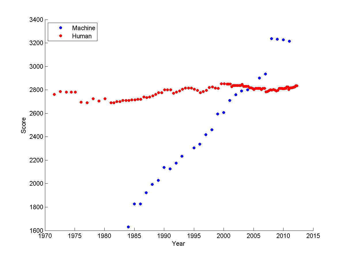 chess Elo ratings over time
from
Sarah Constantin
chess Elo ratings over time
from
Sarah Constantin
Games come in a wide range of types. Questions that affect the choice of computer algorithm include ...
Some other important properties:
What is zero sum? Final rewards for the two (or more) players sum to a constant. That is, a gain for one player involves equivalent losses for the other player(s) This would be true for games where there are a fixed number of prizes to accumulate, but not for games such as scrabble where the total score rises with the skill of both players.
Normally we assume that the opponent is going to play optimally, so we're planning for the worst case. Even if the opponent doesn't play optimally, this is the best approach when you have no model of the mistakes they will make. If you do happen to have insight into the limitations of their play, those can be modelled and exploited.
Time limits are most obvious for competitive games. However, even in a friendly game, your opponent will get bored and walk away (or turn off your power!) if you take too long to decide on a move.
Many video games are good examples of dyanmic environments. If the changes are fast, we might need to switch from game search to methods like reinforcement learning, which can deliver a fast (but less accurate) reaction.
We'll normally assume zero sum, two players, static, large (but not infinite) time limit. We'll start with deterministic games and then consider stochastic ones.
Game search uses a combination of two methods
The new component is adversarial search. Evaluation of game positions uses classifiers (e.g. neural nets) of the sort we've seen before.
Games are typically represented using a tree. Here's an example (from Mitch Marcus at U. Penn) of a very simple game called Hexapawn, invented by Martin Gardner in 1962.
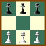
This game uses the two pawn moves from chess (move forwards into an empty square or move diagonally to take an opposing piece). A player wins if (a) he gets a pawn onto the far side, (b) his opponent is out of pawns, or (c) his opponent can't move.
The top of the game tree looks as follows. Notice that each layer of the tree is a ply, so the active player changes between successive levels.

Notice that a game "tree" may contain nodes with identical contents. So we might actually want to treat it as a graph. Or, if we stick to the tree represenation, memoize results to avoid duplicating effort.
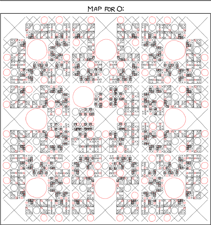
Here's the start of the game tree for a more complex game, tic-tac-toe.
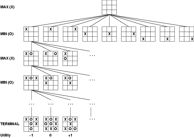
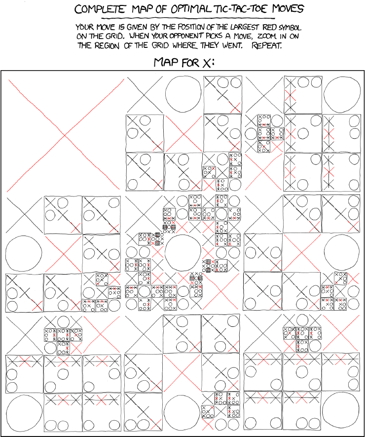
Tic-tac-toe is still simple enough that we can expand out the entire tree of possible moves. It's slightly difficult for humans to do this without making mistakes, but computers are good at this kind of bookkeeping. Here's the details, compacted into a convenient diagram by the good folks at xkcd:
Let's consider how to do adversarial search for a two player, deterministic, zero sum game. For the moment, let's suppose the game is simple enough that we can search whole game tree down to the bottom. Also suppose we expect our opponent to play optimally (or at least close to).
Traditionally we are called max and our opponent is called min. The following shows a (very shallow) game tree for some unspecified game. The final reward values for max are shown at the bottom. Nodes where it's max's turn are often drawn with a triangle pointing up and nodes for min's turns use a triangle pointing down. Here we've labelled the levels instead.
max                             *
                       /        |    \
                  /             |        \
               /                |             \
min        *                    *                 *
          /  \             /    |    \          /   \
max     *      *          *     *     *        *      *
       /|\     |\        /\    /\    /\        |\    /\
      4 2 7    3 1       5 8   2 9   5 6       1 2   3 5
Minimax search propagates values up the tree, level by level. (This can be done with a recursive depth-first search algorithm. At the first level from the bottom, it's max's move. So he picks the highest of the available values:
max                             *
                       /        |    \
                  /             |        \
               /                |             \
min        *                    *                 *
          /  \             /    |    \          /   \
max     7      3          8     9     6        2     5
       /|\     |\        /\    /\    /\        |\    /\
      4 2 7    3 1       5 8   2 9   5 6       1 2   3 5
At the next level (moving upwards) it's min's turn. Min gains when we lose, so he picks the smallest available value:
max                             *
                       /        |    \
                  /             |        \
               /                |             \
min        3                    9                 5
          /  \             /    |    \          /   \
max     7      3          8     9     6        2     5
       /|\     |\        /\    /\    /\        |\    /\
      4 2 7    3 1       5 8   2 9   5 6       1 2   3 5
The top level is max's move, so he again picks the largest value. The double lines show the sequence of moves that will be chosen, if both players play optimally.
max                             6
                       /       ||    \
                  /            ||        \
               /               ||             \
min        3                    6                 2
          /  \             /    |   \\          /   \
max     7      3          8     9     6        2      5
       /|\     |\        /\    /\    /\\       |\    /\
      4 2 7    3 1       5 8   2 9   5 6       1 2   3 5
This procedure is called "minimax" and is optimal against an optimal opponent. Usually our best choice even against suboptimal opponents unless we have special insight into the ways in which they are likely to play badly.
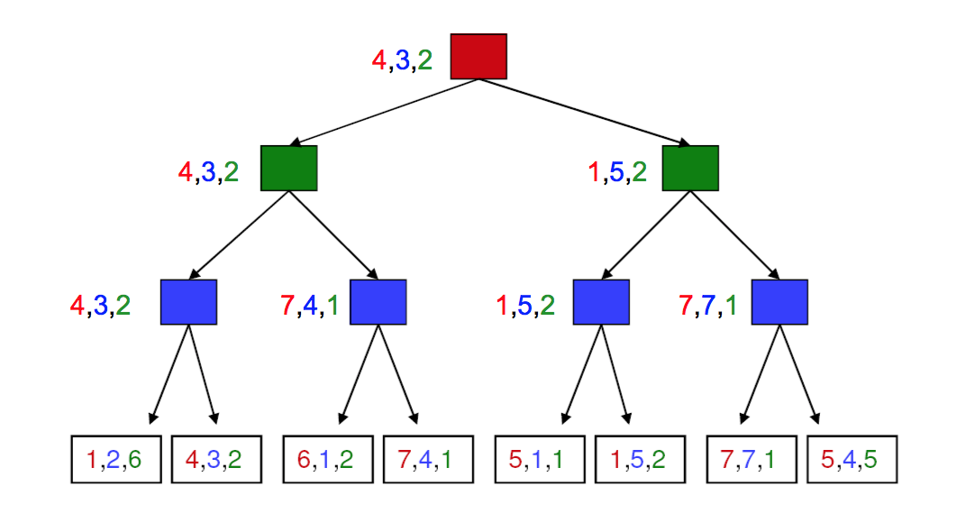
Minimax search extends to cases where we have more than two players and/or the game is not zero sum. In the fully general case, each node at the bottom contains a tuple of reward values (one per player). At each level/ply, the appropriate player choose the tuple that maximizes their reward. The chosen tuples propagate upwards in the tree, as shown below.
For more complex games, we won't have the time/memory required to search the entire game tree. So we'll need to cut off search at some chosen depth. In this case, we heuristically evaluate the game configurations in the bottom level, trying to guess how good they will prove. We then use minimax to propagate values up to the top of the tree and decide what move we'll make.
As play progresses, we'll know exactly what moves have been taken near the top of the tree. Therefore, we'll be able to expand nodes further and further down the game tree.
Evaluating a game configuration usually involves a weighted sum of features. The weights will be learned from databases of played games and/or by playing the AI against itself. Features may be hand-crafted or perhaps learned (e.g. with a deep neural net).
Here's a simple way to evaluate positions for tic-tac-toe. At the start of the game, there are 8 ways to place a line of three tokens. As play progresses, some of these are no longer available to one or both players. So we can evaluate the state by
f(state) = [number of lines open to us] - [number of lines open to opponent]
The figure below shows the evaluations for early parts of the game tree:
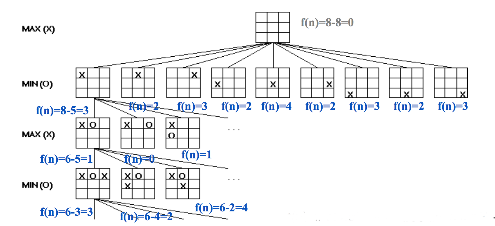 (from Mitch Marcus again)
Evaluations of chess positions dates back to a simple proposal by Alan Turing. In this method, we give a point value to each piece, add up the point values, and consider the difference between our point sum and that of our opponent. Appropriate point values would be
We can do a lot better by considering "positional" features, e.g. whether a piece is being threatened, who has control over the center. A weighted sum of these feature values would be used to evaluate the position. The Deep Blue chess program has over 8000 positional features.
Race matters in face recognition