Pieces of an MDP
When we're in state s, we command an action \( \pi(s) \). However, our buggy controller may put us into a variety of choices for the next state s', with probabilities given by the transition function P.
Bellman equation for best policy
\( U(s) = R(s) + \gamma \max_{a \in A} \sum_{s' \in S} P(s' | s,a)U(s') \)
Recall how we solve the Bellman equation using value iteration. Let \(U_t\) be the utility values at iteration step t.
\( U_{i+1}(s) = R(s) + \gamma \max_{a \in A} \sum_{s' \in S} P(s' | s,a) U_i(s') \)
This can take the gridworld problem (left below) and produce the utility values (right below).
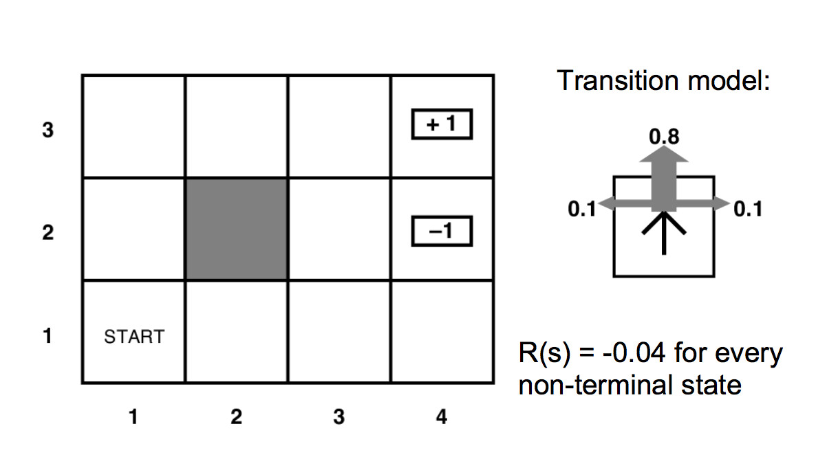
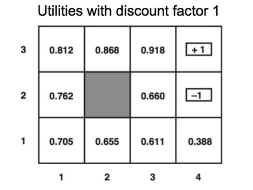
From the final converged utility values, we can read off a final policy (bottom right) by essentially moving towards the neighbor with the highest utility. Taking into account the probabilistic nature of our actions, we get the equation
\( \pi(s) = \text{argmax}_a \sum_{s'} P(s' | s,a) U(s') \)
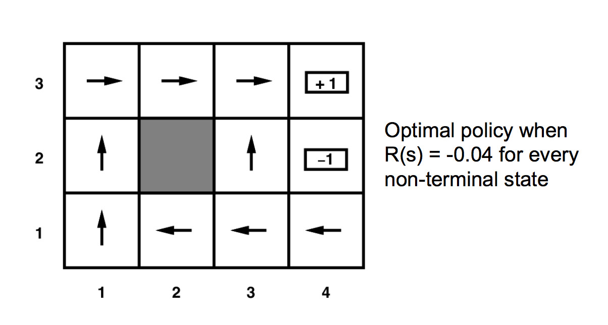
Value iteration eventually converges to the solution. Notice that the optimal utility values are uniquely determined, but there may be one policy consistent with them.
Policy iteration produces the same solution, but faster. It operates as follows:
The values for U and \( \pi \) are closely coupled. Policy iteration makes the emerging policy values explicit, so they can help guide the process of refining the utility values.
We saw above how to convert a set of utility values into a policy. We use this for the "policy evaluation" step. We still need to understand how to do the first (policy evaluation) step.
Our Bellman equation (below) finds the value corresponding to the best action we might take in state s.
\( U(s) = R(s) + \gamma \max_a \sum_{s'} P(s' | s,a)U(s') \)
However, in policy iteration, we already have a draft policy. So we do a similar computation but assuming that we will command action \( \pi(s) \).
\( U(s) = R(s) + \gamma \sum_{s'} P(s' | s, \pi(s)) U(s') \)
We have one of these equations for each state s. The simplification means that each equation is linear. So we have two options for finding a solution:
The value estimation approach is usually faster. We don't need an exact (fully converged) solution, because we'll be repeating this calculation each time we refine our policy \( \pi \).
One useful weak to solving Markov Decision Process is "asynchronous dynamic programming." In each iteration, it's not necessary to update all states. We can select only certain states for updating. E.g.
The details can be spelled out in a wide variety of ways.
So far, we've been solving an MDP under the assumption that we started off knowing all details of P (transition probability) and R (reward function). So we were simply finding a closed form for the recursive Bellman equation. Reinforcement learning (RL) involves the same basic model of states and actions, but our learning agent starts off knowing nothing about P and R. It must find out about P and R (as well as U and \(\pi\)) by taking actions and seeing what happens.
Obviously, the reinforcement learner has terrible performance right at the beginning. The goal is to make it eventually improve to a reasonable level of performance. A reinforcement learning agent must start taking actions with incomplete (initially almost no) information, hoping to gradually learn how to perform well. We typically imagine that it does a very long sequence of actions, returning to the same state multiple types. Its performance starts out very bad but gradually improves to a reasonable level.
A reinforcement learner may be
The latter would be safer for situations where real-world hazards could cause real damage to the robot or the environment.
An important hybrid is "experience replay." In this case, we have an online learner. But instead of forgetting its old experiences, it will
This is a way to make the most use of training experiences that could be limited by practical considerations, e.g. slow, costly, dangerous.
A reinforcement learner repeats the following sequence of steps:
There are two basic choices for the "internal representation":
We'll look at model-free learning next lecture.
A model based learner operates much like a naive Bayes learning algorithm, except that it has to start making decisions as it trains. Initially it would use some default method for picking actions (e.g. random). As it moves around taking actions, it tracks counts for what rewards it got in different states and what state transitions resulted from its commanded actions. Periodically it uses these counts to
Tansition to using our learned policy \(\pi\).
This obvious implementation of a model-based learner tends to be risk-averse. Once a clear policy starts to emerge, it has a strong incentive to stick to its familiar strategy rather than exploring the rest of its environment. So it could miss very good possibilities (e.g. large rewards) if it didn't happen to see them early.
To improve performance, we modify our method of selecting actions:
"Explore" could be implemented in various ways, such as
The probability of exploring would typically be set high at the start of learning and gradually decreased, allowing the agent to settle into a specific final policy.
The decision about how often to explore must depend on the state s. States that are easy to reach from the starting state(s) end up explored very early, when more distant states may have barely been reached. For each state s, it's important to continue doing significant amounts of exploration until each action has been tried (in s) enough times to have a clear sense of what it does.