Gridworld pictures are from the U.C. Berkeley CS 188 materials (Pieter Abbeel and Dan Klein) except where noted.

Reinforcement Learning

Reinforcement learning is a technique for deciding which action to take in an environment where your feedback is delayed and your knowledge of the environment is uncertain. Reinforcement Learning can be used on a variety of AI tasks, notably board games. But it is frequently associated with learning how to control mechanical systems. For example, a long-standing reinforcement learning task is pole balancing.

Markov Decision Processes

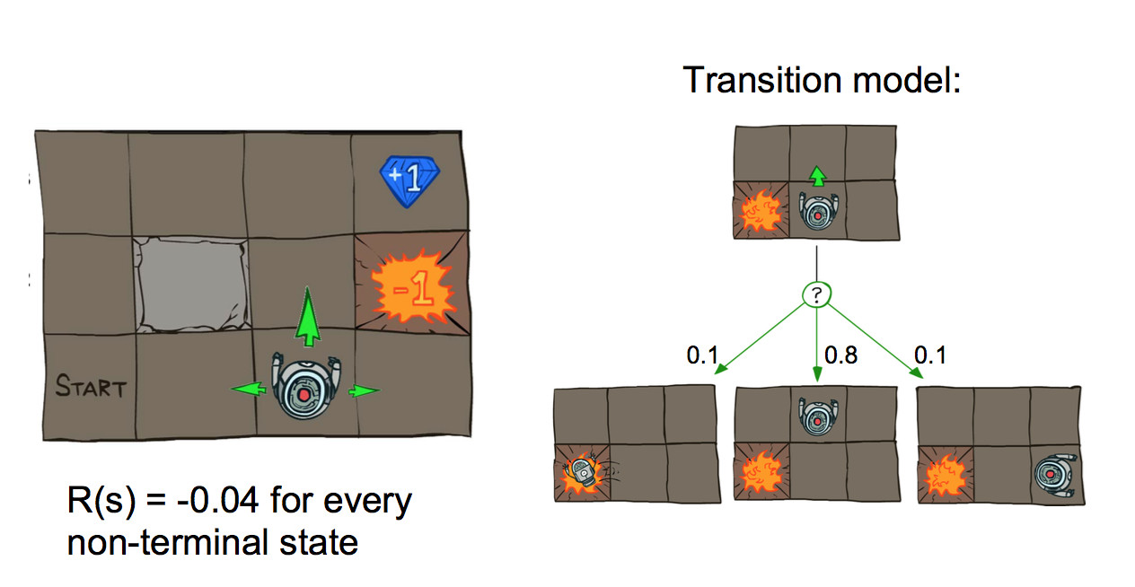
The environment for reinforcement learning is typically modelled as a Markov Decision Process (MDP). The basic set-up is an agent (e.g. imagine a robot) moving around a world like the one shown below. Positions add or deduct points from your score. The Agent's goal is to accumulate the most points.

It's best to imagine this as a game that goes on forever. Many real-world games are finite (e.g. a board game) or have actions that stop the action (e.g. robot falls down the stairs). We'll assume that reaching an end state will automatically reset you back to the start of a new game, so the process continues forever.

Actions are executed with errors. So if our agent commands a forward motion, there's some chance that they will instead move sideways. In real life, actions might not happen as commanded due to a combination of errors in the motion control and errors in our geometrical model of the environment.

Mathematical setup

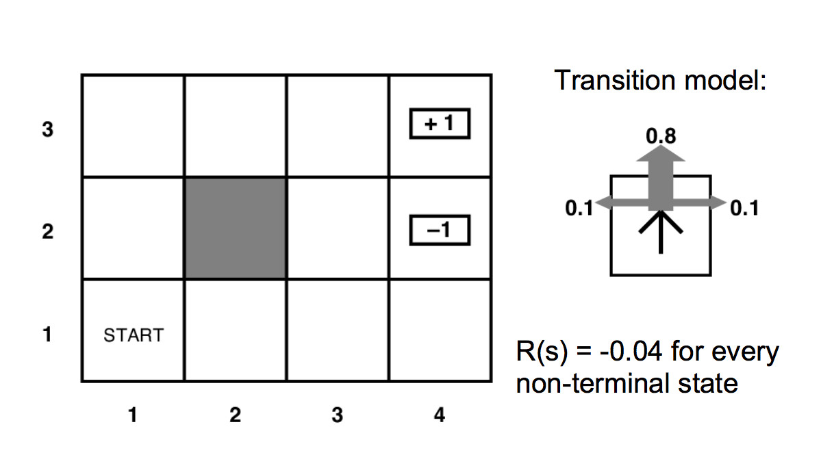
Eliminating the pretty details gives us a mathematician-friendly diagram:

Our MDP's specification contains

• set of states $s \in S$
• set of actions $a \in A$
• reward function R(s)
• transition function P(s' | s,a)

The transition function tells us the probability that a commanded action a in a state s will cause a transition to state s'.

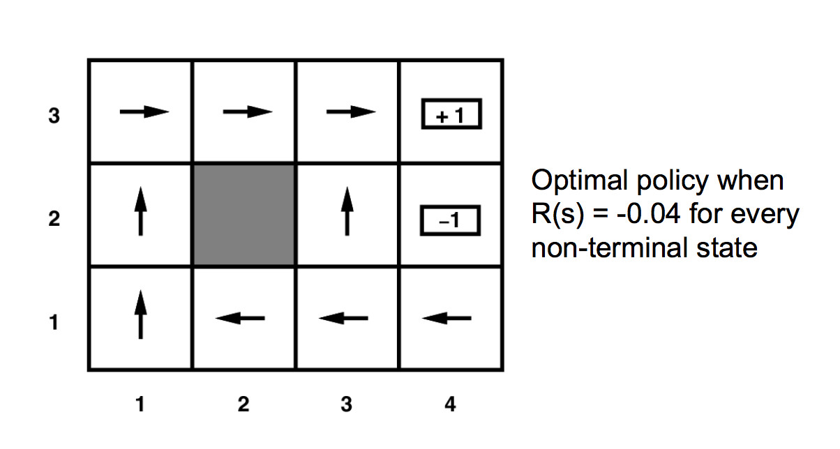
Our solution will be a policy $\pi(s)$ which specifies which action to command when we are in each state. For our small example, the arrows in the diagram below show the optimal policy.

The reward function

The reward function could have any pattern of negative and positive values. However, the intended pattern is

• A few states have big rewards or negative consequences.
• The rest of the states have some small background reward, often constant across all of these background states.

For our example above, the unmarked states have reward -0.04.

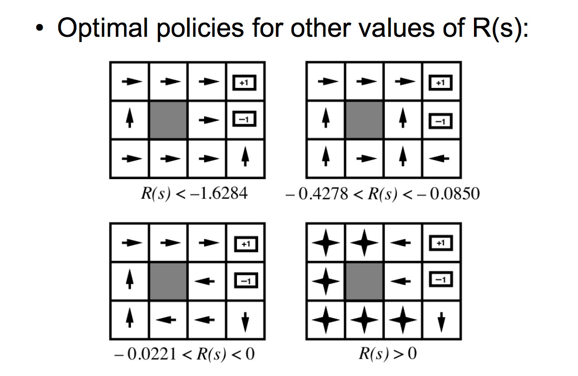
The background reward for the unmarked states changes the personality of the MDP. If the background reward is high (lower right below), the agent has no strong incentive to look for the high-reward states. If the background is strongly negative (upper left), the agent will head aggressively for the high-reward states, even at the risk of landing in the -1 location.

What makes a policy good?

We'd like our policy to maximize reward over time. So something like the sum of

P(sequence)R(sequence)

over all sequences of states, where R(sequence) is the total reward for the sequence of states. P(sequence) is how often this sequence of states happens.

However, sequences of states might be extremely long or (for the mathematicians in the audience) infinitely long. Our agent needs to be able to learn and react in a reasonable amount of time. Worse, infinite sequences of values might not necessarily converge to finite values, even with the sequence probabilities taken into account.

So we make the assumption that rewards are better if they occur sooner. The equations in the next section will define a "utility" for each state that takes this into account. The utility of a state is based on its own reward and, also, on rewards that can be obtained from nearby states. That is, being near a big reward is almost as good as being at the big reward.

So what we're actually trying to maximize is

P(sequence)U(sequence)

U(sequence) is the sum of the utilities of the states in the sequence and P(sequence) is how often this sequence of states happens.

The Bellman equation

Suppose our actions were deterministic, then we could express the utility of each state in terms of the utilities of adjacent states like this:

$U(s) = R(s) + \max_{a \in A} U(move(a,s))$

where move(a,s) is the state that results if we perform action a in state s. We are assuming that the agent always picks the best move (optimal policy).

Since our action does not, in fact, entirely control the next state s', we need to compute a sum that's weighted by the probability of each next state. The expected utility of the next state would be $\sum_{s'\in S} P(s' | s,a)U(s')$, so this would give us a recursive equation

$U(s) = R(s) + \max_{a \in A} \sum_{s'\in S} P(s' | s,a)U(s')$

The actual equation should also include a reward delay multiplier $\gamma$. Downweighting the contribution of neighboring states by $\gamma$ causes their rewards to be considered less important than the immediate reward R(s). It also causes the system of equations to converge. So the final "Bellman equation" looks like this:

$U(s) = R(s) + \gamma \max_{a \in A} \sum_{s'\in S} P(s' | s,a)U(s')$

Specifically, this is the Bellman equation for the optimal policy.

Short version of why it converges. Since our MDP is finite, our rewards all have absolute value $\le$ some bound M. If we repeatedly apply the Bellman equation to write out the utility of an extended sequence of actions, the kth action in the sequence will have a discounted reward $\le \gamma^k M$. So the sum is a geometric series and thus converges if $0 \le \gamma < 1$.

The Bellman equation for a fixed policy

Suppose that we have picked some policy $\pi$. Then the Bellman equation for this fixed policy is simpler because we know exactly what action we'll command:

$U(s) = R(s) + \gamma \sum_{s'\in S} P(s' | s,\pi(s))U(s')$

Our goal is to find the best policy. This is tightly coupled to finding a closed form solution to the Bellman equation, i.e. an actual utility value for each state. Once we know the utilities, the best policy is move towards the neighbors with the highest utility.

Solving the MDP

There's a variety of ways to solve MDP's and closely-related reinforcement learning problems:

• Value iteration
• Policy iteration
• Dynamic methods that look a lot like perceptron training

Value iteration

The simplest solution method is value iteration. This method repeatedly applies the Bellman equation to update utility values for each state. Suppose $U_k(s)$ is the utility value for state s in iteration k. Then

• initialize $U_1(s) =$ for all states s
• loop for k = 1 until the values converge
  • $U_{k+1}(s) = R(s) + \gamma \max_{a \in A} \sum_{s'\in S} P(s' | s,a)U_k(s')$

These slides show how the utility values change as the iteration progresses. The final output utilities and the corresponding policy are shown below.

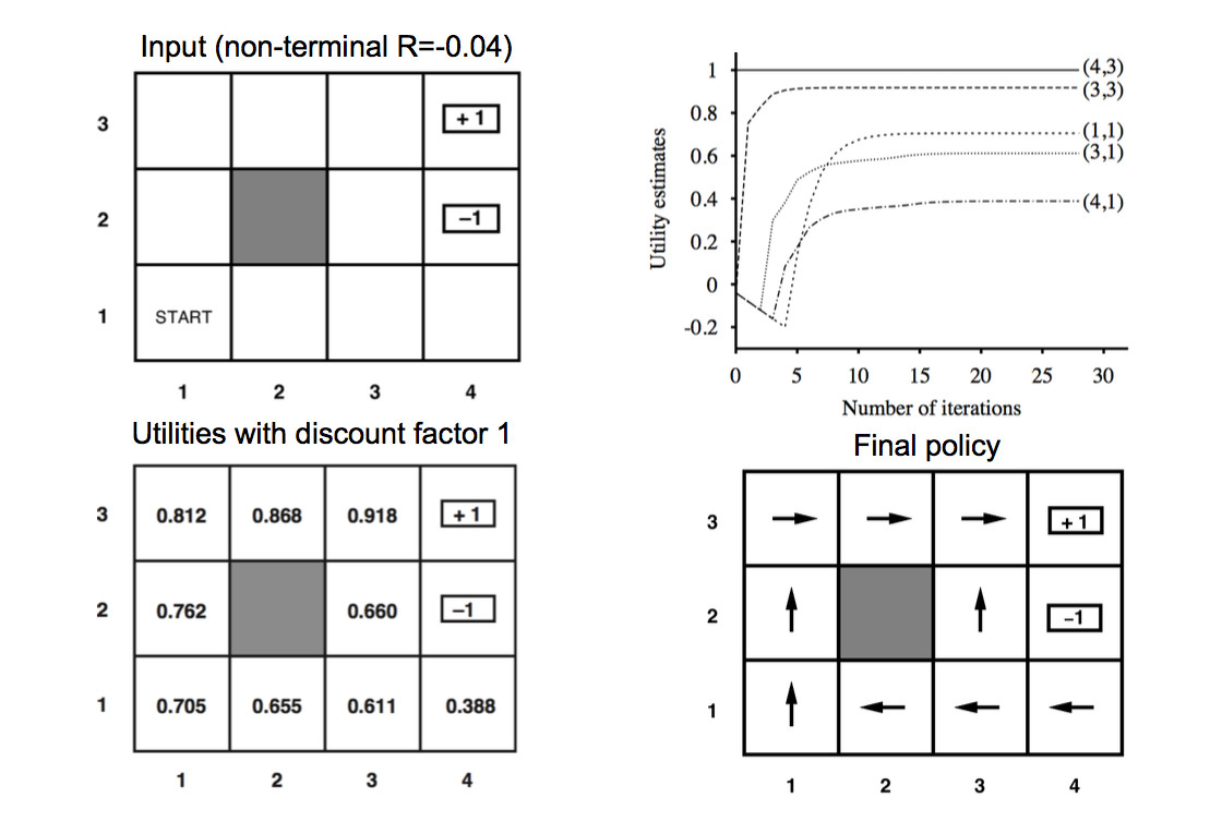
We can read a policy off the final utility values: move towards the highest-utility neighbor.

You can play with a larger example in Andrej Karpathy's gridworld demo.

Warning: Notational variant

Some authors (notably the Berkeley course) use variants of the Bellman equation like this:

$V(s) = \max_a \sum_{s}' P(s' | s,a) [R(s,a,s') + \gamma V(s')]$

There is no deep change involved here. This is partly just pushing around the algebra. Also, passing more arguments to the reward function R allows a more complicated theory of rewards, i.e. depending not only on the new state but also the previous state and the action you used. If we use our simpler model of rewards, then this V(s) these can be related to our U(s) as follows

U(s) = R(s) + V(s)

AI in action

Self-driving car can't see jaywalkers