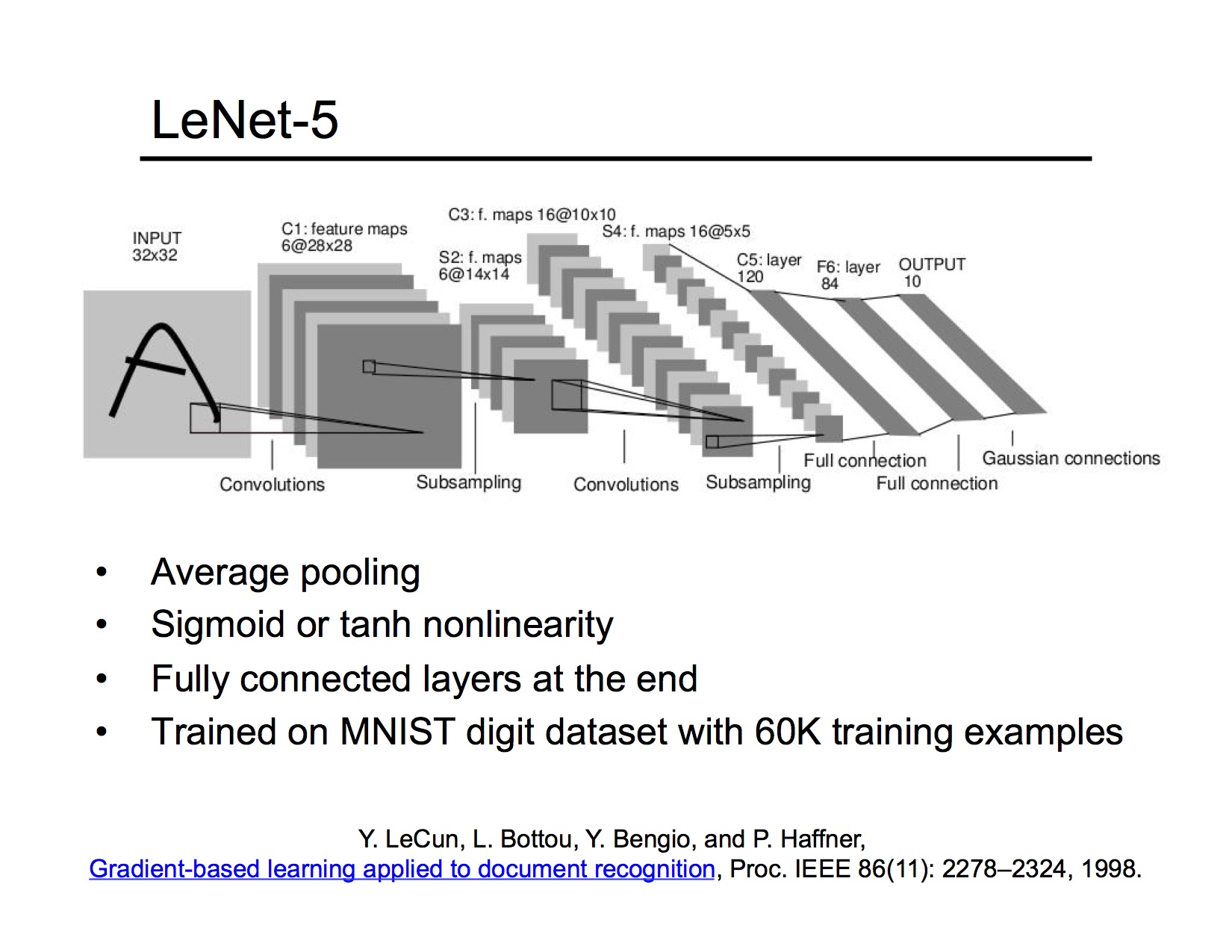
Recall our neural net example from last lecture:
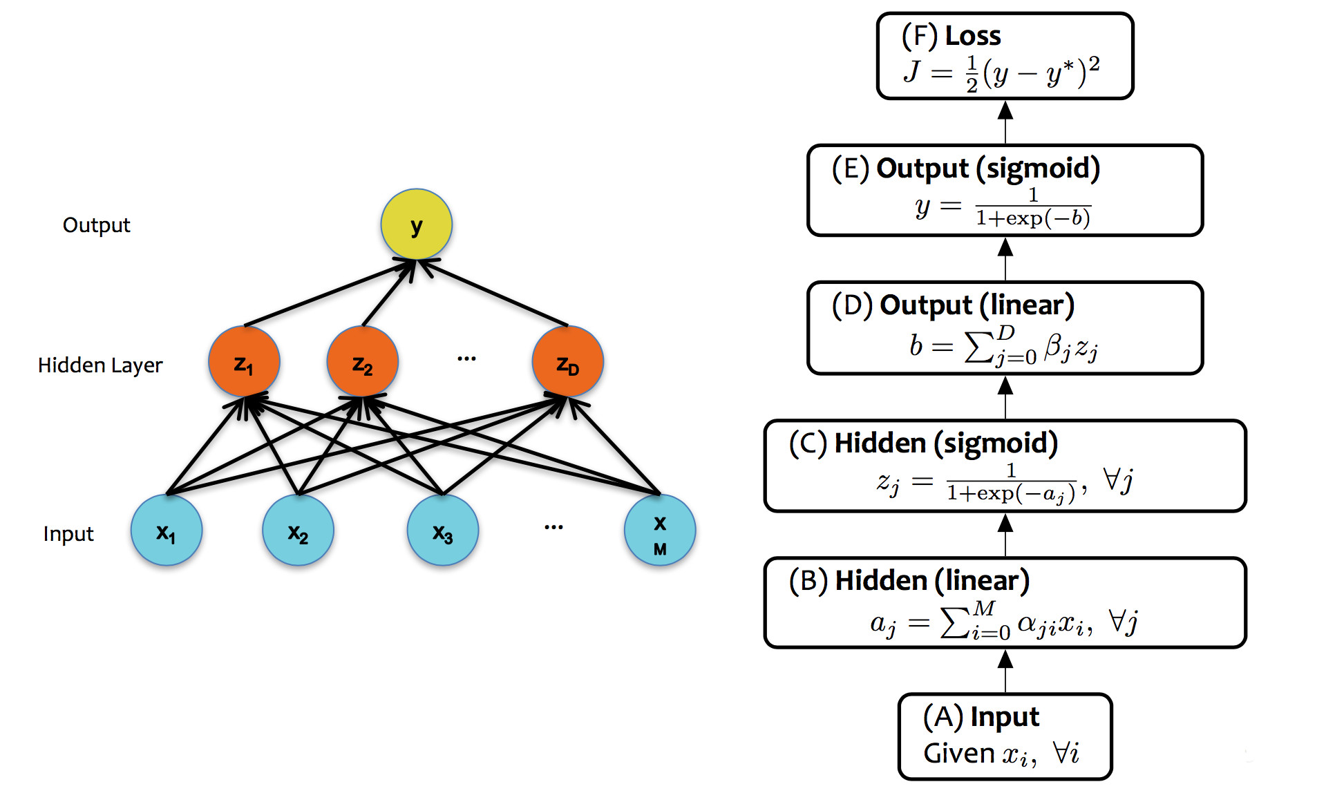
from Matt Gormley
For each training pair, our update algorithm looks like:
The diagram below shows the forward and backward values for this network:
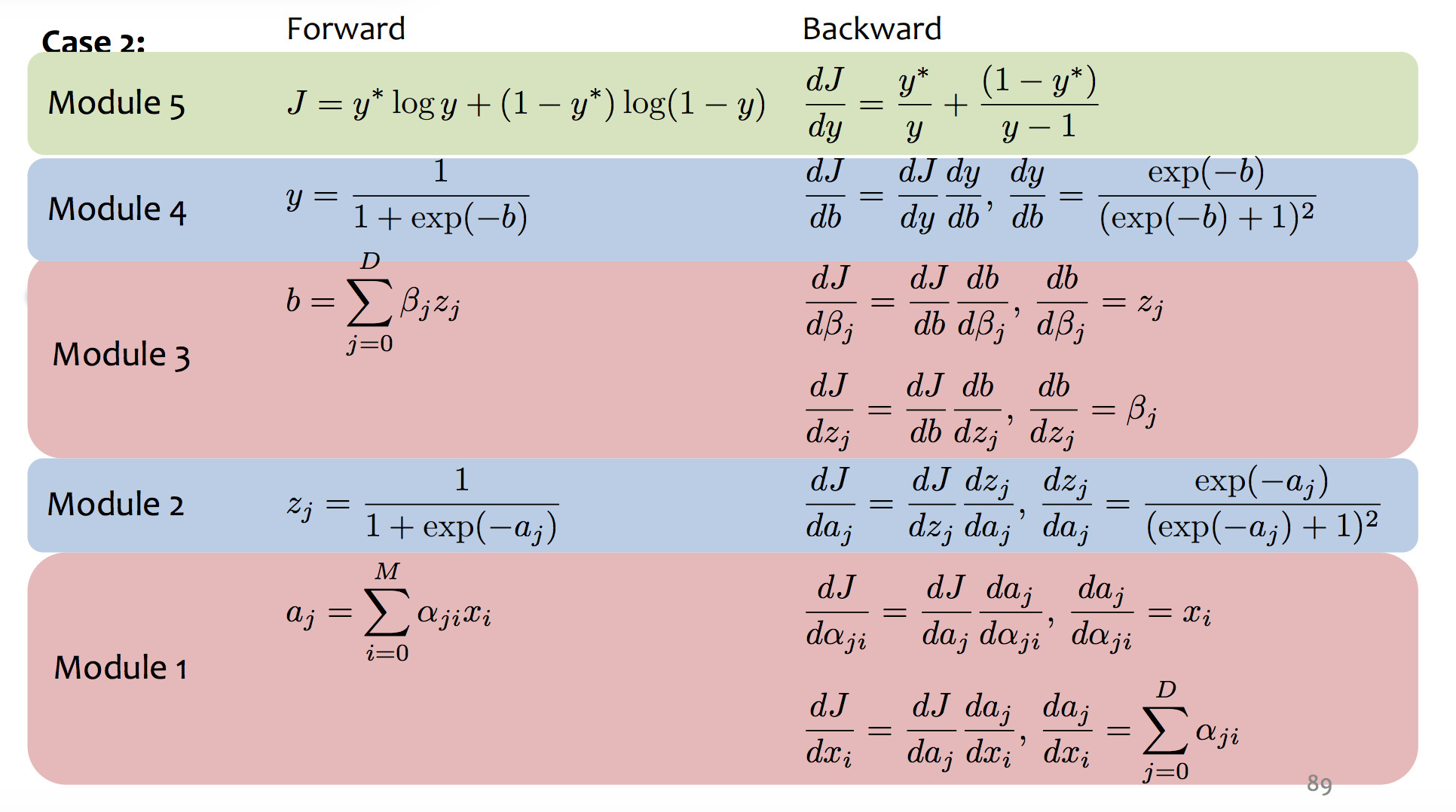 (from Matt Gormley)
Backpropagation is essentially a mechanical exercise in applying the chain rule repeatedly. Humans make mistakes, and direct manual coding will have bugs. So, as you might expect, computers have taken over most of the work as they for (say) register allocation. Read the very tiny example in Jurafsky and Martin (7.4.3 and 7.4.4) to get a sense of the process, but then assume you'll use TensorFlow or PyTorch to make this happen for a real network.
Unfortunately, training neural nets is somewhat of a black art because the process isn't entirely stable. Three issues are prominent:
Perceptron training works fine with all weights initialized to zero. This won't work in a neural net, because each layer typically has many neurons connected in parallel. We'd like parallel units to look for complementary features but the naive training algorithm will cause them to have identical behavior. At that point, we might as well economize by just having one unit. Two approaches to symmetry breaking:
One specific proposal for randomization is dropout: Within the network, each unit pays attention to training data only with probability p. On other training inputs, it stops listening and starts reading its email or something. The units that aren't asleep have to classify that input on their own. This can help prevent overfitting.
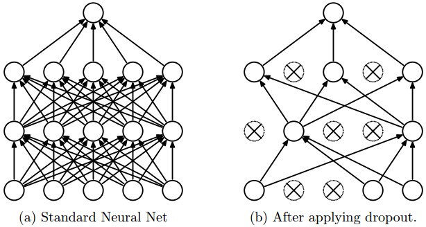
from Srivastava et al.
Neural nets infamously tend to tune themselves to peculiarities of the dataset. This kind of overfitting will make them less able to deal with similar real-world data. The dropout technique will reduce this problem. Another method is Data augmentation.
Data augmentation tackles the fact that training data is always very sparse, but we have additional domain knowledge that can help fill in the gaps. We can make more training examples by perturbing existing ones in ways that shouldn't (ideally) change the network's output. For example, if you have one picture of a cat, make more by translating or rotating the cat. See this paper by Taylor and Nitschke.
In order for training to work right, gradients computed during backprojection need to stay in a sensible range of sizes. A sigmoid activation function only works well when output numbers tend to stay in the middle area that has a significant slope.
The underflow/overflow issues happen because numbers that are somewhat too small/large tend to become smaller/larger.
Several approaches to mitigating this problem, none of which looks (to me) like a solid, complete solution.
Convolutional neural nets are a specialized architecture designed to work well on image data (also apparently used somewhat for speech data). Images have two distinctive properties:
The large size of each layer makes it infeasible to connect units to every unit in the previous layer. Full interconnection can be done for artificially small (e.g. 32x32) input images. For larger images, this will create too many weights to train effectively with available training data. For physical networks (e.g. the human brain), there is also a direct hardware cost for each connection.
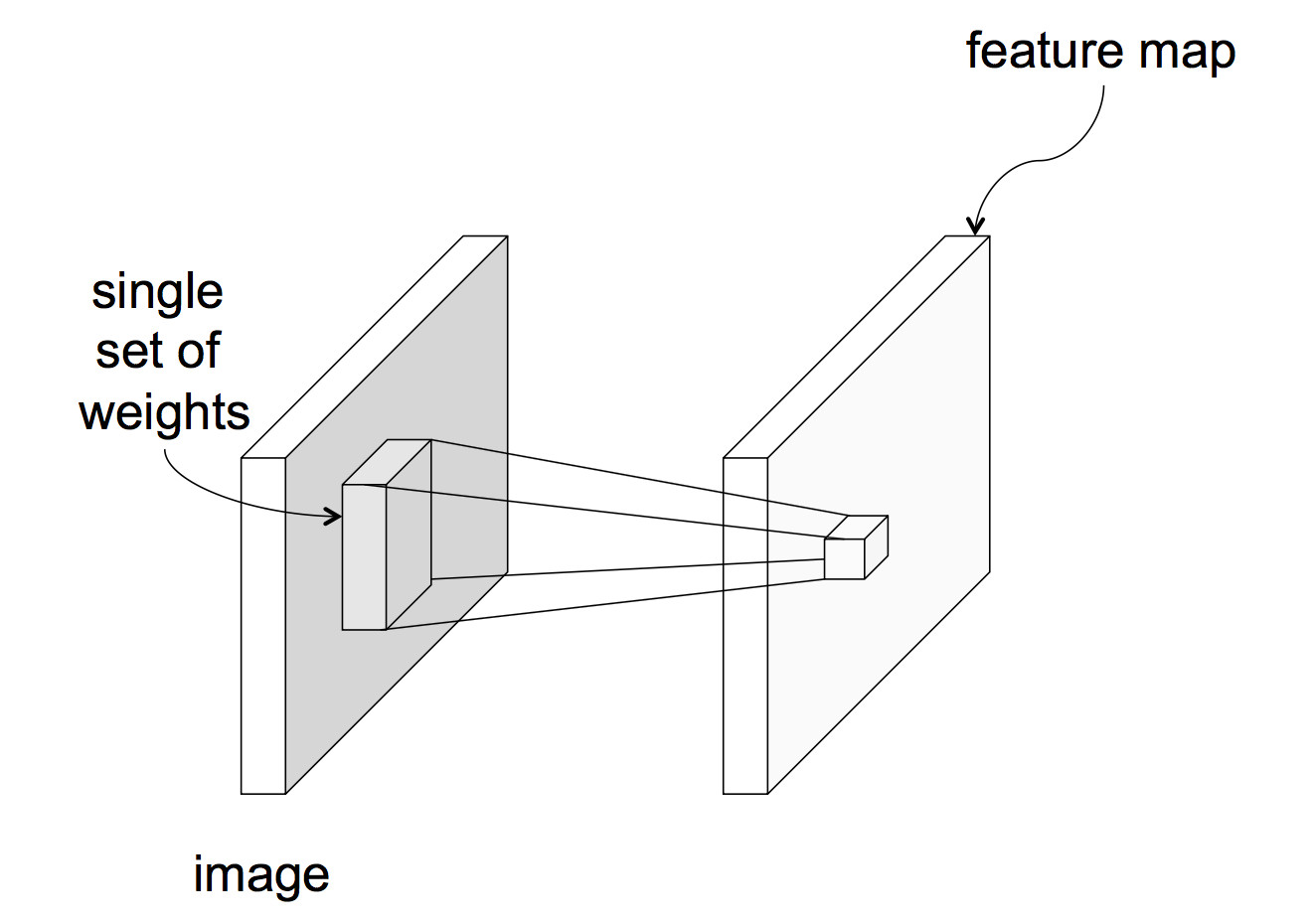
In a CNN, each unit reads input only from a local region of the preceding layer:
 from Lana Lazebnik Fall 2017
This means that each unit computes a weighted sum of the values in that local region. In signal processing, this is known as "convolution" and the set of weights is known as a "mask." To get a sense of what you can do with small convolution operations, play with this convolution demo (by Zoltan Fegyver). For example, the following mask will locate sharp edges in the image:
              0 -1  0
             -1  4 -1
              0 -1  0
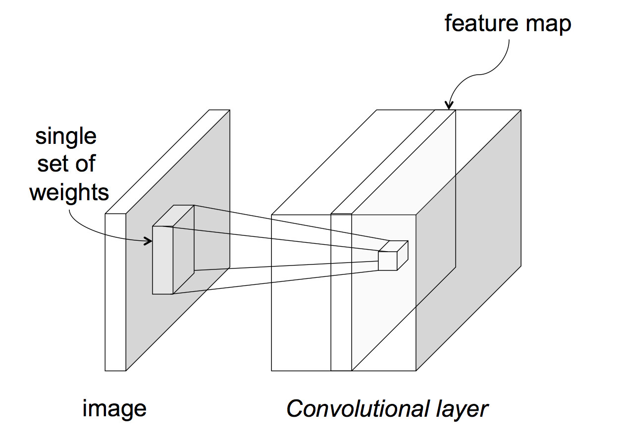
The above picture assumes that each layer of the network has only one value at each (x,y) position. This is typically not the case. An input image often has three values (red, green, blue) at each pixel. Going from the input to the first hidden layer, one might imagine that a number of different convolution masks would be useful to apply, each picking out a different type of feature. So, in reality, each network layer has a significant thickness, i.e. a number of different values at each (x,y) location.
 from Lana Lazebnik Fall 2017
This animation from Andrej Karpathy shows how one layer of processing might work:
In this example, each unit is producing values only at every third input location. So the output layer is a 3x3 image, with has two values at each (x,y) position.
Two useful bits of jargon:
Some CNN's use "parameter sharing": units in the same layer share a common set of weights and bias. This cuts down on the number of parameters to train. May worsen performance if different regions in the input images are expected to have different properties, e.g. the object of interest is always centered.
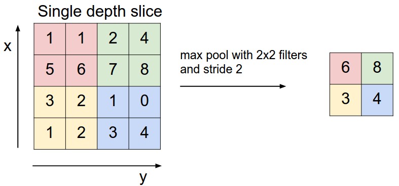
A third type of neural net layer reduces the size of the data, by producting an output value only for every kth input value in each dimension. This is called a "pooling" layer. The output values may be either selected input values, or the average over a group of inputs, or the maximum over a group of inputs.
 from
Andrej Karpathy
from
Andrej Karpathy
This kind of reduction in size ("downsampling") is especially sensible when data values are changing only slowly across the image. For example, color often changes very slowly except at object boundaries, and the human visual system represents color at a much lower resolution than brightness.
A complete CNN typically contains three types of layers