Recap

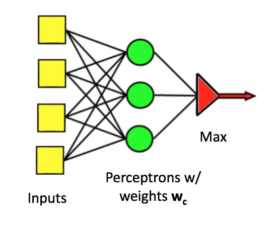
Recall: a classifier unit consists of

• the weighted sum of input feature values
• the activation function
• the loss function

For a percetron, the activation function is the sign function. We use 0/1 loss, i.e. we lose one point for each wrong output.

For a differentiable unit, the activation function might be the ReLU function or the sigmoid function. Recall the equation for the sigmoid function: $\sigma(x) = \frac{1}{1 + e^{-x}}$ The loss function might be the L2 norm or cross-entropy.

Softmax

Recall how we built a multi-class perceptron: join their outputs together with an argmax to select the class with the highest output. We'd like to do something similar with differentiable units.

(from Mark Hasegawa-Johnson, CS 440, Spring 2018)

There is no (reasonable) way to produce a single output variable that takes discrete values (one per class). So we use a "one-hot" representation of the correct output. A one-hot representation is a vector with one element per class. The target class gets the value 1 and other classes get zero. E.g. if we have 8 classes and we want to specify the third one, our vector will look like:

[0, 0, 1, 0, 0, 0, 0, 0]

One-hot doesn't scale well to large sets of classes, but works well for medium-sized collections.

Now, suppose we have a sequence of classifier outputs, one per class. $v_1,\ldots,v_n$. We often have little control over the range of numbers in the $v_i$ values. Some might even be negative. We'd like to map these outputs to a one-hot vector. Softmax is a differentiable function that approximates this discrete behavior. It's best thought of as a version of argmax.

Specifically, softmax maps each $v_i$ to $\displaystyle \frac{e^{v_i}}{\sum_i e^{v_i}}$. The exponentiation accentuates the contrast between the largest value and the others, and forces all the values to be positive. The denominator normalizes all the values into the range [0,1], so they look like probabilities (for folks who want to see them as probabilities).

Regularization

Any type of model fitting is subject to possible overfitting. When this seems to be creating problems, a useful trick is "regularization." Suppose that our set of training data is T. Then, rather than minimizing loss(model,T), we minimize

loss(model,T) + $\lambda$ * complexity(model)

The right way to measure model complexity depends somewhat on the task. A simple method for a linear classifier would be $\sum_i (w_i)^2$, where the $w_i$ are the classifier's weights. Recall that squaring makes the L2 norm sensitive to outlier (aka wrong) input values. In this case, this behavior is a feature: this measure of model complexity will pay strong attention to unusually large weights and make the classifier less likely to use them. Linguistic methods based on "minimumum description length" are using a varint of the same idea.

$\lambda$ is a constant that balances the desire to fit the data with the desire to produce a simple model. This is yet another parameter that would need to be tuned experimentally using our development data. The picture below illustrates how the output of a neural net classifier becomes simpler as $\lambda$ is increased. (The neural net in this example is more complex, with hidden units.)

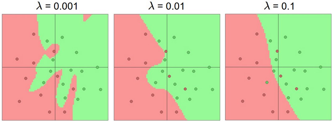from Andrej Karpathy course notes

Credits to Matt Gormley are from 10-601 CMU 2017

Hidden layers

So far, we've seen some systems containing more than one classifier unit, but each unit was always directly connected to the inputs and an output. When people say "neural net," they usually mean a design with more than layer of units, including "hidden" units which aren't directly connected to the output. Early neural nets tended to have at most a couple hidden layers (as in the picture below). Modern designs typically use many layers.

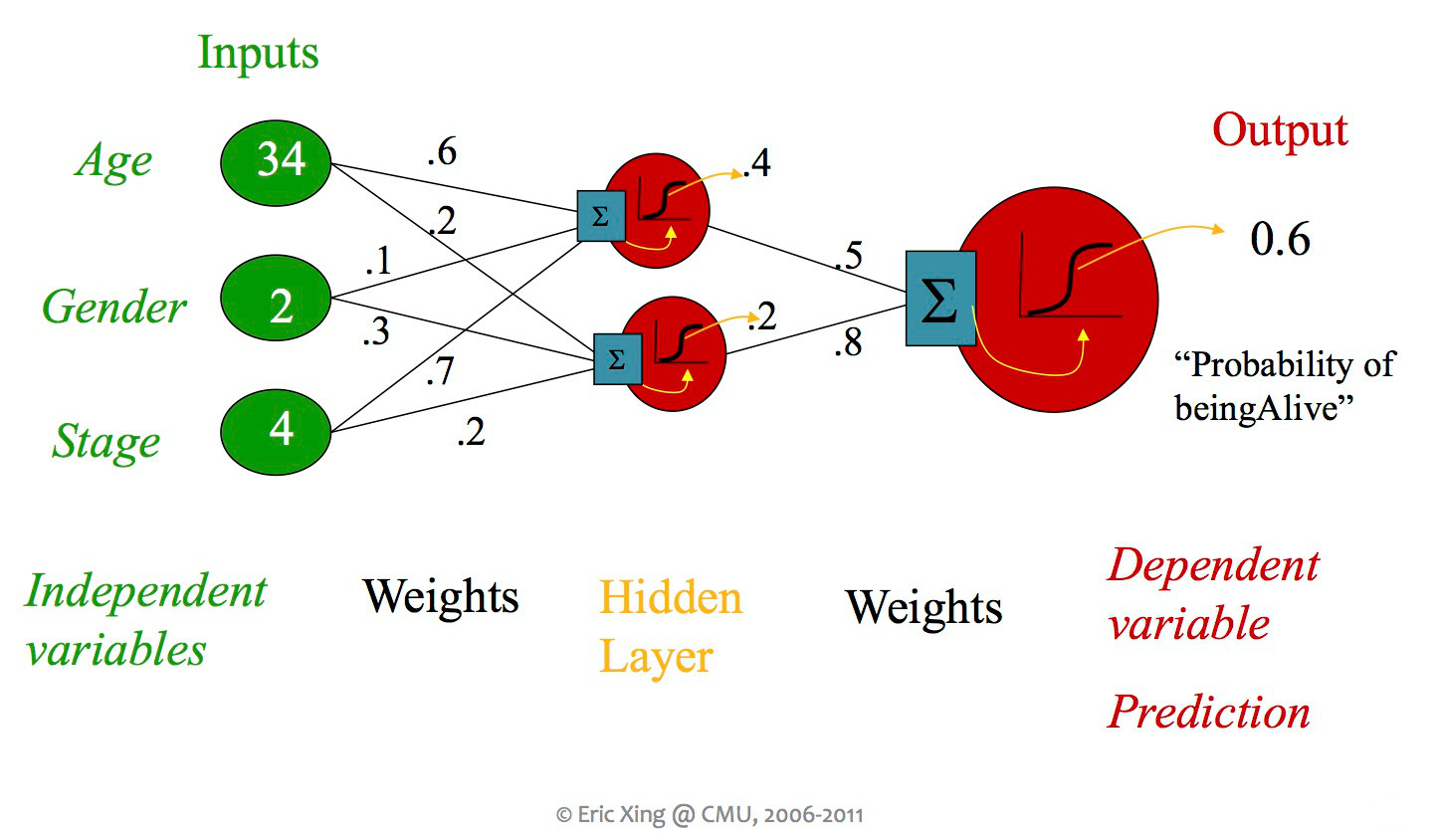
from Eric Xing via Matt Gormley

A single unit in a neural net can look like any of the linear classifiers we've seen previously. Moreover, different layers within a neural net design may use types of units (e.g. different activation functions). However, modern neural nets typically use entirely differentiable functions, so that gradient descent can be used to tune the weights.

from Matt Gormley

The core ideas in neural networks go back decades. Some of their recent success is due to better understanding of design and/or theory. But perhaps the biggest reasons have to do with better hardware and better library support for the annoying mechanical parts.

Deep networks

In theory, a single hidden layer is sufficient to approximate any continuous function, assuming you have enough hidden units. However, deeper neural nets seem to be easier to design and train. These deep networks normally emulate the layers of processing found in previous human-designed classifiers. So each layer transforms the input so as to make it more sophisticated ("high level"), compacts large inputs (e.g. huge pictures) into a more manageable set of features, etc. The picture below shows a face recognizer in which the bottom units detect edges, later units detect small pieces of the face (e.g. eyes), and the last level (before the output) finds faces.

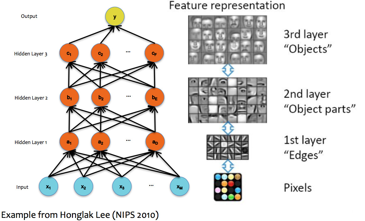
(from Matt Gormley)

Here's a set of slides showing a prettier version of the same kind of layer visualization. These are from Lana Lazebnik based on M. Zeiler and R. Fergus Visualizing and Understanding Convolutional Networks

Approximating functions

Here are some slides showing how a neural net with increasingly many layers can approximate increasingly complex decision boundaries. (from Eric Postma via Jason Eisner via Matt Gormley)

To approximate a complex shape with only 2-3 layers, each hidden unit takes on some limited task. For example, one unit may define the top edge of a set of examples lying in a band:

• Approximating a diagonal band (from Matt Gormley)
• Approximating a "pocket" (from Matt Gormley)

More complex shapes such as this two "pocket" region (pictures from Matt Gormley) require increasingly many layers. Notice that the second picture shows k-nearest neighbors on the same set of data. K-nearest neighbors does well as this kind of task. It's just not very efficient for large numbers of points, esp. in high dimensions.

Training: high level idea

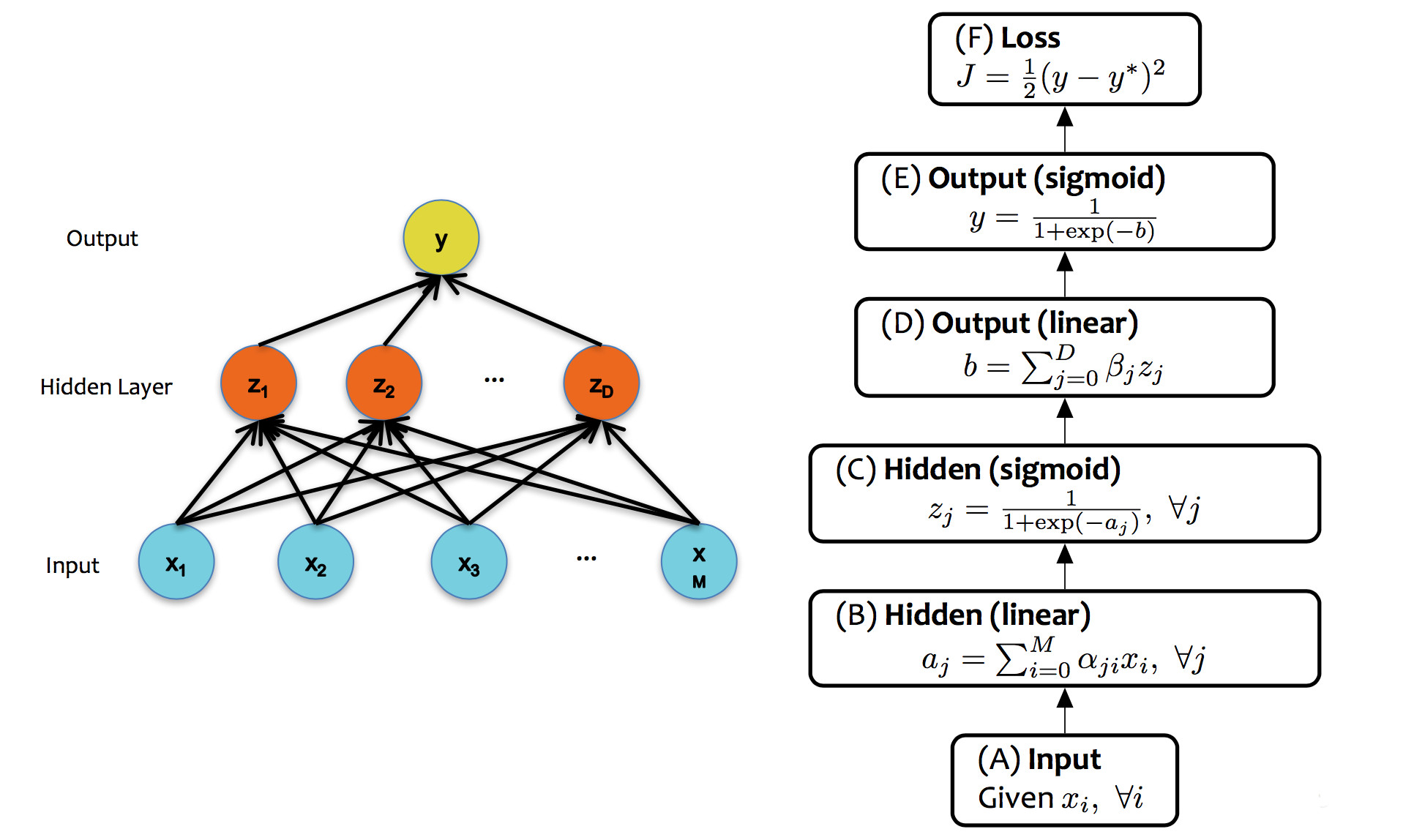
Neural nets are trained in much the same way as individual classifiers. That is, we initialize the weights, then sweep through the input data multiple types updating the weights. When we see a training pair, we updated the weights, moving each weight $w_i$ in the direction that decreases the loss:

$w_i = w_i - \alpha * \frac{\partial \text{ loss}}{\partial w_i}$

Notice that the loss is available at the output end of the network, but the weight $w_i$ might be in an early layer. So the two are related by a chain of composed functions, often a long chain of functions. We have to compute the derivative of this composition.

Review: the chain rule

Remember the chain rule from calculus. If $h(x) = f(g(x))$, the chain rule says that $h'(x) = f'(g(x))*g'(x)$. In other words, to compute $h'(x)$, we'll need the derivatives of the two individual functions, plus the value of of them applied to the input.

Let's write out the same thing in Liebniz notation, with some explicit variables for the intermediate results:

• y = g(x)
• z = f(y) = f(g(x))
• chain rule: $\frac{dz}{dx} = \frac{dz}{dy} * \frac{dy}{dx}$

This version of the chain rule now looks very simple: it's just a product. However, we need to remember that it depends implicitly on the equations defining y in terms of x, and z in terms of y. Let's use the term "forward values" for values like y and z.

We can now see that the derivative for a whole composed chain of functions is, essentially, the product of the derivatives for the individual functions. So, for a weight w at some level of the network, we can assemble the value for $\frac{d\text{ loss}}{dw}$ using

• the derivative of each individual function
• the chain rule: multiply those derivatives
• the forward values: substitute to eliminate all the intermediate variables

Neural net update

Now, suppose we have a training pair ($\vec{x}, y')$. (y' is the correct class for $\vec{x}$.) Updating the neural net weights happens as follows:

• Forward pass: starting from the input $\vec{x}$, calculate the output values for all units. We work forwards through the network, using our current weights.
• Suppose the final output is y. We put y and y' into our loss function to calculate the final loss value.
• Backpropagation: starting from the loss at the end of the network and working backwards, calculate how changes to each weight will affect the loss. This combines the derivatives of each individual function with the values from the forward pass.

Next class, we'll work through a brief example. There's another in Jurafsky and Martin (7.4.3 and 7.4.4). The details of backpropagation are a huge pain to work through by hand. In practice, this is done by libraries such PyTorch or Tensorflow.

AI in action

A project to physically model networks of neurons.