Basic perceptron

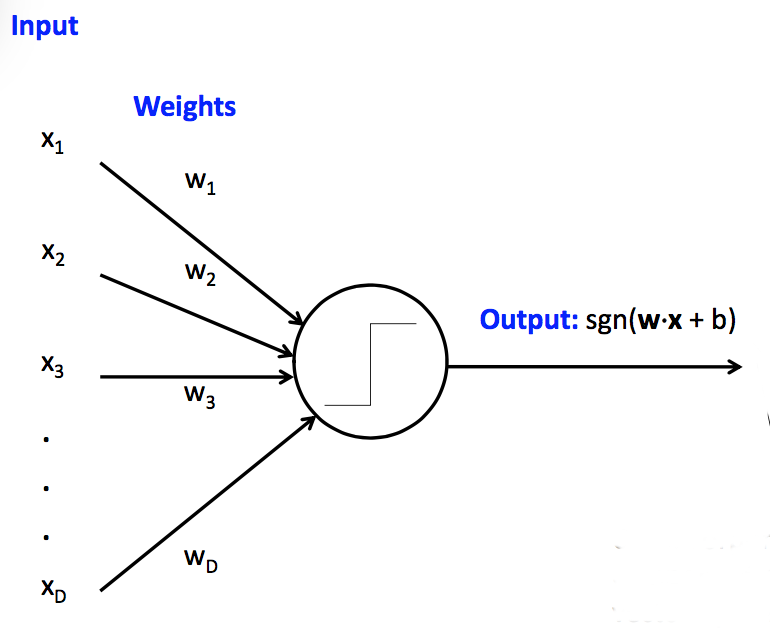
Recall our basic model of a linear unit. This particular one is a perceptron, because its activation function returns a bindary value (1 or -1). Perceptrons have limited capabilities but are particularly easy to learn

(from Mark Hasegawa-Johnson, CS 440, Spring 2018)

The training process

So far, we've assumed that the weights $w_1,\ldots, w_n$ and the bias term were given to us by magic. In practice, they are learned from training data.

Suppose that we have a set T of training data pairs (x,y), where x is a feature vector and y is the (correct) class label. Our training algorithm looks like:

• Initialize weights to zero
• For each training example (x,y), update the weights to improve the changes of classifying x correctly.

Perceptron Learning Rule

Let's suppose that our unit is a classical perceptron, i.e. our activation function is the sign function. Then we can update the weights using the "perceptron learning rule". Suppose that x is a feature vector, y is the correct class label, and y' is the class label that was computed using our current weights. Then our update rule is:

• If y' = y, do nothing.
• Otherwise $w_i = w_i + \alpha * y * x_i$

The "learning rate" constant $\alpha$ controls how quickly the update process changes in response to new data.

There's several variants of this equation, e.g.

$w_i = w_i + \alpha * (y-y') * x_i$

When trying to understand why they are equivalent, notice that the only possible values for y and y' are 1 and -1. So if $y = y'$, then $(y-y')$ is zero and our update rule does nothing. Otherwise, $(y-y')$ is equal to either 2 or -2, with the sign matching that of the correct answer (y). The factor of 2 is irrelevant, because we can tune $\alpha$ to whatever we wish.

This training procedure will converge if

• data are linearly separable or
• we throttle the size of the updates as training proceeds by decreasing $\alpha$.

Apparently convergence is guaranteed if the learning rate is proportional to $\frac{1}{t}$ where t is the current iteration number. The book recommends a gentler formula: make $\alpha$ proportional to $\frac{1000}{1000+t}$.

Processing the training data

One run through training data through the update rule is called an "epoch." One generally uses multiple epochs, i.e. the algorithm sees each training pair several times.

Datasets often have strong local correlations, because they have been formed by concatenating sets of data (e.g. documents) that each have a strong topic focus. So it's often best to process the individual training examples in a random order.

Limitations

Perceptrons can be very useful but have significant limitations.

• The decision boundary can only be a line

  Fixes:

  • use multiple units (neural net)
  • massage input features

• If there is overlap between the two categories, can thrash between different boundary positions.

  Fixes:

  • reduce learning rate as learning progresses
  • don't update weights any more than needed to fix mistake in current example
  • cap the maximum change in weights (e.g. this example may have been a mistake)

• If there is a gap between the two categories, uncertain where to place the boundary line.

  Fix: look at "support vector machines" (SVM's). The big idea for an SVM is that only examples near the boundary matter. So we try to maximize the distance between the closest sample point and the boundary (the "margin").

Multi-class perceptrons

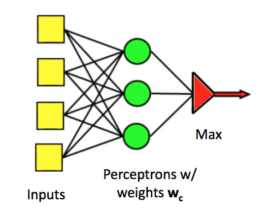
Perceptrons can easily be generalized to produce one of a set of class labels, rather than a yes/no answer. We use several parallel classifier units. Each has its own set of weights. Join the individual outputs into one output using argmax (i.e. pick the class that has the largest output value).

(from Mark Hasegawa-Johnson, CS 440, Spring 2018)

Update rule: Suppose we see (x,y) as a training example, but our current output class is y'. Update rule:

• Do nothing to the units for classes other than y and y'.
• Each weight in class y: $w_i = w_i + \alpha * x_i$
• Each weight in class y': $w_i = w_i - \alpha * x_i$

The classification regions for a multi-class perceptron look like the picture below. That is, each pair of classes is separated by a linear boundary. But the region for each class is defined by several linear boundaries.

from Wikipedia

Differentiable units

Classical perceptrons have a step function activation function, so they return only 1 or -1. Our accuracy is the count of how many times we got the answer right. When we generalize to multi-layer networks, it will be much more convenient to have a differentiable output function, so that we can use gradient descent to update the weights.

To do this, we need to separate two functions at the output end of the unit:

• the activation function: our model of uncertainty about the decision
• the loss function: the penalty for getting the decision wrong.

Our whole classification function is the composition of three functions:

• the weighted sum of input feature values
• the activation function
• the loss function

In a multi-layer network, there will be activation functions at each layer and one loss function at the very end.

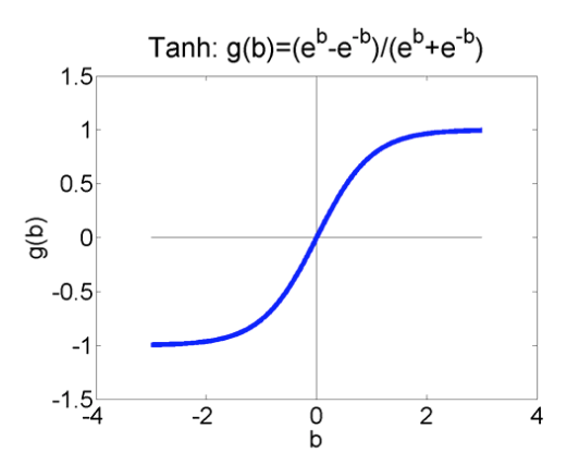
The activation function for a perceptron is a step function: 1 above the threshold, -1 below it.. Popular choices for differentiable activation functions are

• logistic(x) (also called a sigmoid) $\frac{1}{(1+e^{-x})}$
• tanh $\frac{e^x - e^{-x}}{e^x + e^{-x}}$ (see below)
• rectified linear unit (ReLU): f(x) = x when positive, f(x) = 0 if negative

from Mark Hasegawa-Johnson

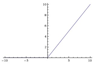RelU function from Andrej Karpathy course notes.

The loss function for a perceptron is "zero-one loss". We get 1 for each wrong answer, 0 for each correct one. Suppose that y is the correct output and p is the output of our activation function. Popular differentiable loss functions include

• L2 norm: (y-p)^2
• cross-entropy loss: -(y log p + (1-y)log(1-p))

In all cases, we average these losses over all our training pairs.

When using the L2 norm to measure distances, one normally takes the square of each individual error, adds them all up, and then takes the square root of the result. In our case, we can lose the square root because it doesn't affect the minimization. (If f(x) is non-negative, $\sqrt{f(x)}$ has a minimum when f(x) does.) The quantity we are trying to minimize is the sum of the squared errors over all the training input pairs. So, when looking at one individual pair, we just square the error for that pair.

Recall that entropy is the number of bits required to (optimally) compress a pool of values. The high-level idea of cross-entropy is that we have built a model of probabilities (e.g. using some training data) and then use that model to compress a different set of data. Cross-entropy measures how well our model succeeds on this new data. This is one way to measure the difference between the model and the new data.

Excessively comprehensive lists if you are curious

• activation functions
• loss functions

Example of differentiable updating

Let's assume we use the logistic/sigmoid for our activation function and the L2 norm for our loss function. (See details in Russell and Norvig, 18.6.)

To work out the update rule for learning weight values, suppose we have a training example (x,y). The output with our current weights is $f_w(x) = \sigma(w*x)$ where $\sigma$ is the sigmoid function. Our loss function is $loss(w,x): (y - f_w(x))^2$.

For gradient descent, we adjust our weights in the direction of the gradient. That is, our update rule should look like:

$w_i = w_i - \alpha * \frac{ \partial \text{loss(w,x)}}{\partial w_i}$

To figure out the formula for $\frac{ \partial \text{loss(w,x)}}{\partial w_i}$, we apply the chain rule, look up the derivative of the logistic function, and set $y' = f_w(x)$ to make the equation easier to read. See Russell and Norvig 18.6 for the derivation. This gives us an update rule:

$w_i = w_i + \alpha * (y - y') * y' * (1- y') * x_i$

Ugly, unintuitive, but straightforward to code.