Recal: a classifier maps input examples (each a set of feature values) to class labels. Our task is to train a model on a set of examples with labels, and then assign the correct labels to new input examples.
Training and testing can be interleaved to varying extents
Feedback may be more or less direct
Here's a schematic representation of English vowels (from Wikipedia). From this, you might reasonable expect to experimental data to look like several tight clusters of points, well-separated. If that were true, then classification would be easy: model each cluster with a regeion of simple shape (e.g. ellipse), compare a new sample to these region, and pick the one that contains it.
However, experimental datapoints for these vowels (even after some normalization) actually look more like the following. If we can't improve the picture by clever normalization (sometimes possible), we need to use more robust methods of classification.
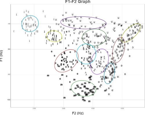
(These are the tirst two formants of English vowels by 50 British speakers, normalized by the mean and standard deviation of each speaker's productions. From the Experimental Phonetics course PALSG304 at UCL.)
We'll see four types of classifiers:
A decision tree makes its decision by asking a series of questions. For example, here is a a decision tree user interface for identifying vines (by Mara Cohen, Brandeis University). The features, in this case, are macroscopic properties of the vine that are easy for a human to determine, e.g. whether it has thorns. The top levels of this tree look like
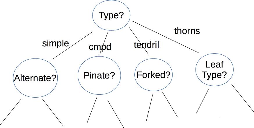
Depending on the application, the nodes of the tree may ask yes/no questions, multiple choice (e.g. simple vs. complex vs. tendril vs thorns), or set a threshold on a continuous space of values (e.g. is the tree below or above 6' tall?). The output label may be binary (e.g. is this poisonous?), from a small set (edible, other non-poisonous, poisonous), or from a large set (e.g. all vines found in Massachusetts).
Here's an example of a tree created by thresholding two continuous variable values (from David Forsyth, Applied Machine Learning). Notice that the split on the second variable (x) is different for the two main branches.

Each node in the tree represents a pool of examples. Ideally, each leaf node contains only objects of the same type. However, that isn't always true if the classes aren't cleanly distinguished by the available features (see the vowel picture above). So, when we reach a leaf node, the algorithm returns the most frequent label in its pool.
If we have enough decision levels in our tree, we can force each pool to contain objects of only one type. However, this is not a wise decision. Deep trees are difficult to construct (see the algorithm in Russell and Norvig) and prone to overfitting their training data. It is more effective to create a "forest" of shallow trees (bounded depth) and have these trees vote on the best label to return. The set of shallow trees is created by choosing variables and possible split locations randomly.
Whether we're building a deep or shallow tree, some possible splits are a bad idea. For example, the righthand split leaves us with two half-size pools that are no more useful than the original big pool.
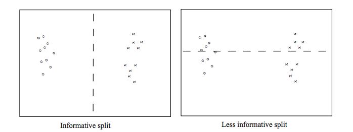
(From David Forsyth, Applied Machine Learning.)
A good split should produce subpools that are less diverse than the original pool. If we're choosing between two candidate splits (e.g. two thresholds for the same numerical variable), it's better to pick the one that produces subpools that are more uniform. Diversity/uniformity is measured using entropy.
Suppose that we are trying to compress English text, by translating each character into a string of bits. We'll get better compression if more frequent characters are given shorter bit strings. For example, the table below shows the frequencies and Huffman codes for letters in a toy example from Wikipedia.
| Char | Freq | Code | Char | Freq | Code | Char | Freq | Code | Char | Freq | Code | Char | Freq | Code | Char | Freq | Code | Char | Freq | Code |
|---|---|---|---|---|---|---|---|---|---|---|---|---|---|---|---|---|---|---|---|---|
| space | 7 | 111 | a | 4 | 010 | e | 4 | 000 | ||||||||||||
| f | 3 | 1101 | h | 2 | 1010 | i | 2 | 1000 | m | 2 | 0111 | n | 2 | 0010 | s | 2 | 1011 | t | 2 | 0110 |
| l | 1 | 11001 | o | 1 | 00110 | p | 1 | 10011 | r | 1 | 11000 | u | 1 | 00111 | x | 1 | 10010 |
Suppose that we have a (finite) set of letter types S. Suppose that M is a finite list of letters from S, with each letter type (e.g. "e") possibly included more than once in M. Each letter type c has a probability P(c) (i.e. its fraction of the members of M). An optimal compression scheme would require \(\log(\frac{1}{P(c)}) \) bits in each code. (All logs in this discussion are base 2.)
To understand why this is plausible, suppose that all the characters have the same probability. That means that our collection contains \(\frac{1}{P(c)} \) different characters. So we need \(\frac{1}{P(c)} \) different codes, therefore \(\log(\frac{1}{P(c)}) \) bits in each code. For example, suppose S has 8 types of letter and M contains one of each. Then we'll need 8 distinct codes (one per letter), so each code must have 3 bits. This squares with the fact that each letter has probability 1/8 and \(\log(\frac{1}{P(c)}) = \log(\frac{1}{1/8}) = \log(8) = 3 \).
The entropy of the list M is the average number of bits per character when we replace the letters in M with their codes. To compute this, we average the lengths of the codes, weighting the contribution of each letter c by its probability P(c). This give us
\( H(M) = \sum_{c \in S} P(c) \log(\frac{1}{P(c)}) \)
Recall that \(\log(\frac{1}{P(c)}) = -\log_2(P(c))\). Applying this, we get the standard form of the entropy definition.
\( H(M) = - \sum_{c \in S} P(c) \log(P(c)) \)
In practice, good compression schemes don't operate on individual characters and also they don't achieve this theoretical optimum bit rate. However, entropy is a very good way to measure the homogeneity of a collection of discrete values, such as the values in the decision tree pools.
For more information, look up Shannon's source coding theorem.
Another way to classify an input example is to find the most similar training example and copy its label.
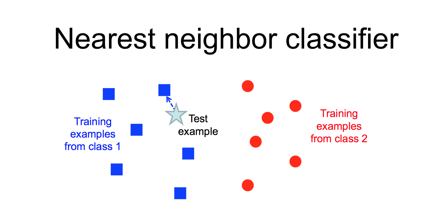 from Lana Lazebnik
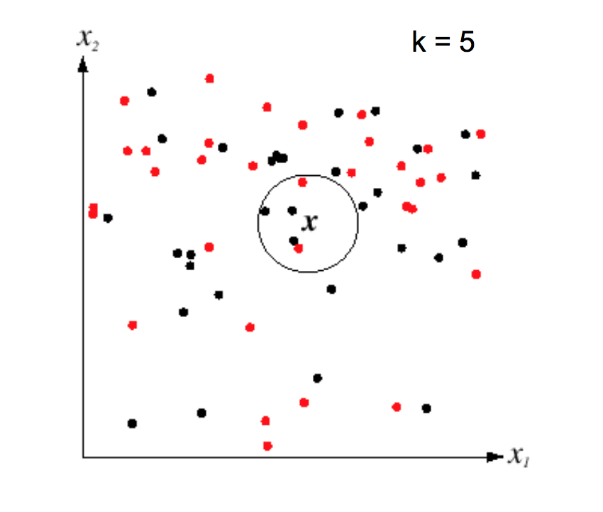
This "nearest neighbor" method is prone to overfitting, especially if the data is messy and so examples from different classes are somewhat intermixed. However, performance can be greatly improved by finding the k nearest neighbors for some small value of k (e.g. 5-10).
 from Lana Lazebnik
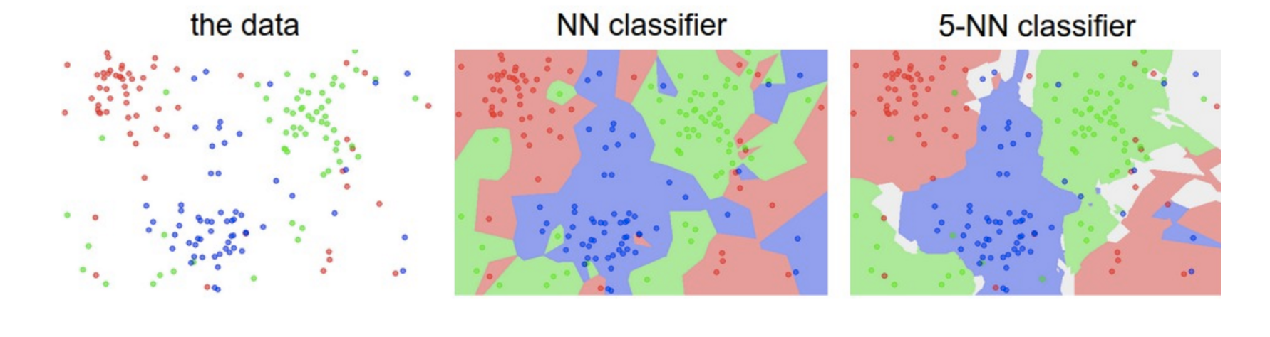
K nearest neighbors can model complex patterns of data, as in the following picture. Notice that larger values of k smooth the classifier regions, making it less likely that we're overfitting to the training data.
 from Andrej Karpathy
A limitation of k nearest neighbors is that the algorithm requires us to remember all the training examples, so it takes a lot of memory if we have a lot of training data. In low dimensions, a k-D tree can be used to find efficiently find the nearest neighbors for an input example. However, efficiently handling higher dimensions is more tricky and beyond the scope of this course.
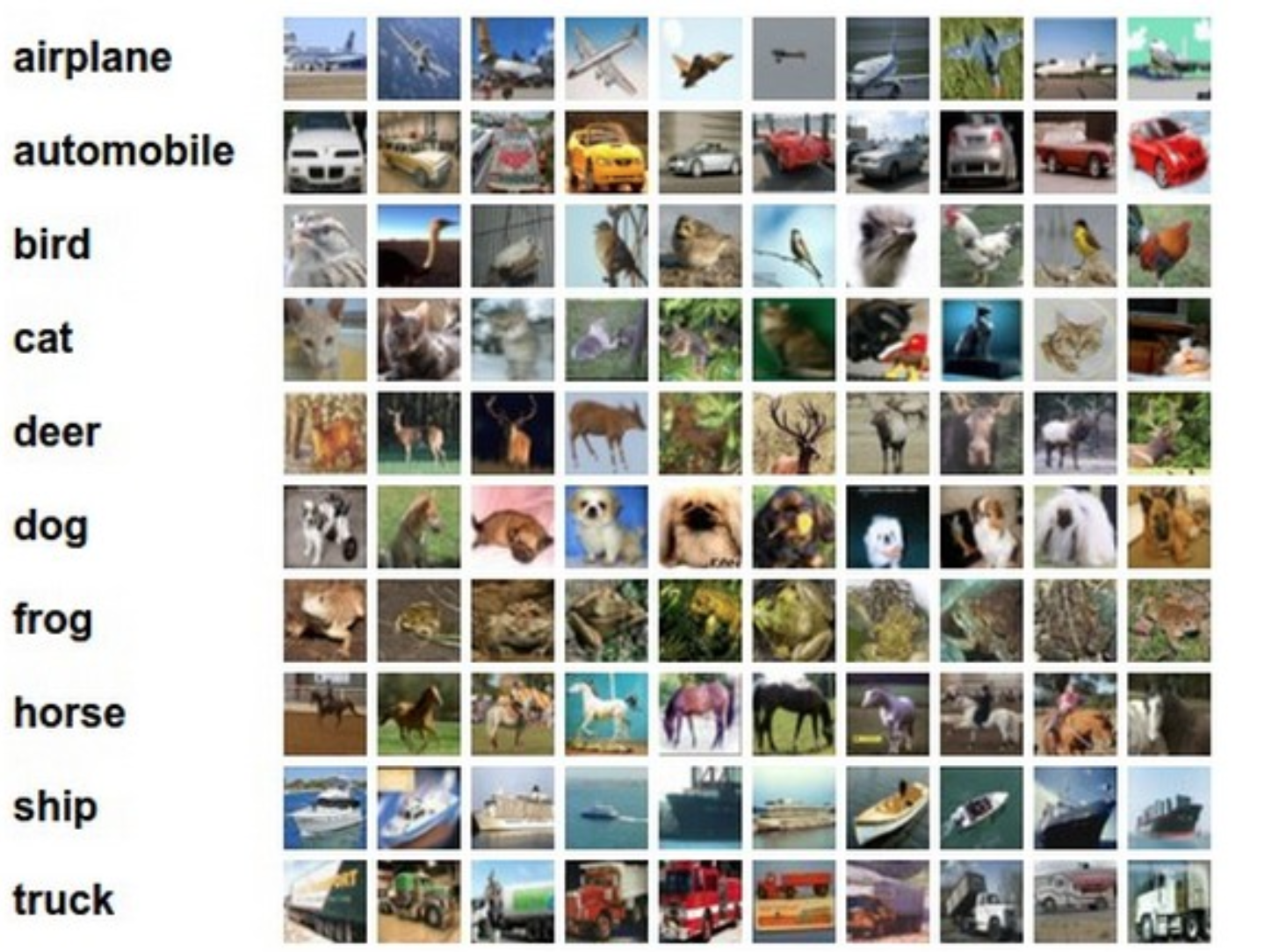
This method can be applied to somewhat more complex types of examples. Consider the CFAR-10 dataset below. (Pictures are from Andrej Karpathy cs231n course notes.) Each image is 32 by 32, with 3 color values at each pixel. So we have 3072 feature values for each example image.
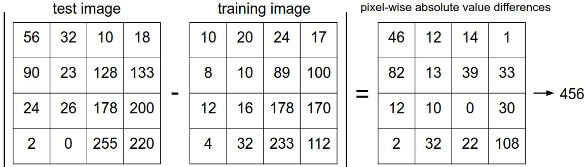
We can calculate the distance between two examples by subtracting corresponding feature values. Here is a picture of how this works for a 4x4 toy image.
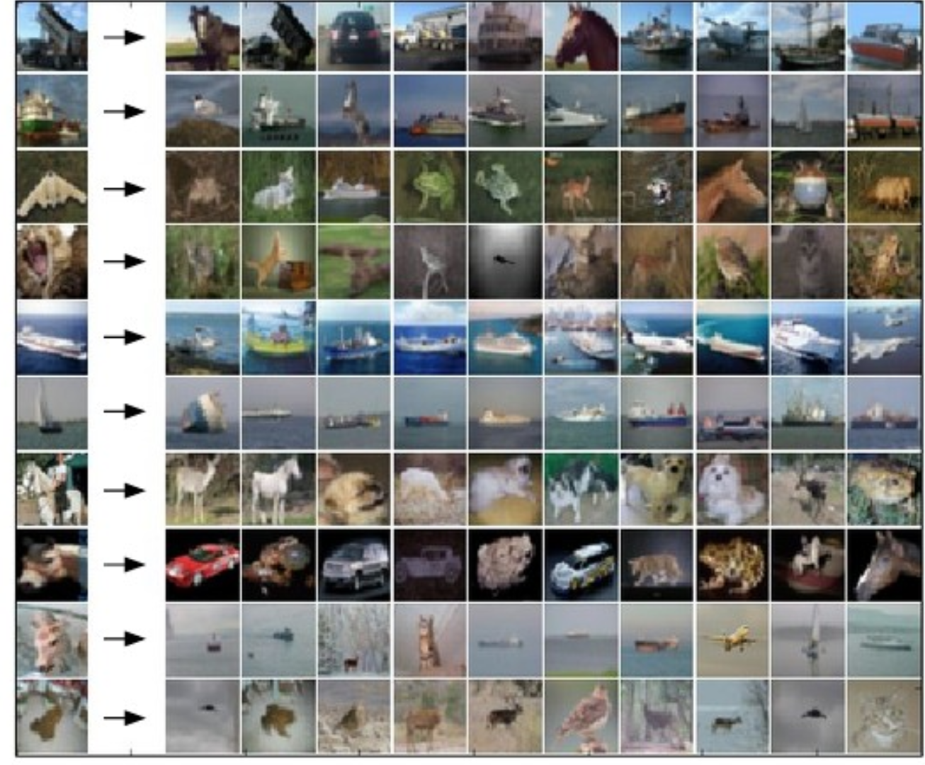
The following picture shows how some sample test images map to their 10 nearest neighbors.
More precisely, suppose that \(\vec{x}\) and \(\vec{y}\) are two feature vectors (e.g. pixel values for two images). Then there are two different simple ways to calculate the distance between two feature vectors:
As we saw with A* search for robot motion planning, the best choice depends on the details of your dataset. The L1 norm is less sensitive to outlier values. The L2 norm is continuous and differentiable, which can be handy for certain mathematical derivations.
GAN learning to hide data so it can cheat on a learning task.
