Each word has several possible tags, with different probabilities.

• in principle, if we had perfect knowledge of English
• as seen in our training set

For example, "can" appears using in several roles:

• Monica can swim. (modal verb)
• A can of beans. (noun)
• I will can the beans. (verb)

Some other words with multiple uses

• cover: noun, verb, adjective (cover crop)
• over: preposition, noun (e.g. cricket)
• pot: noun, verb

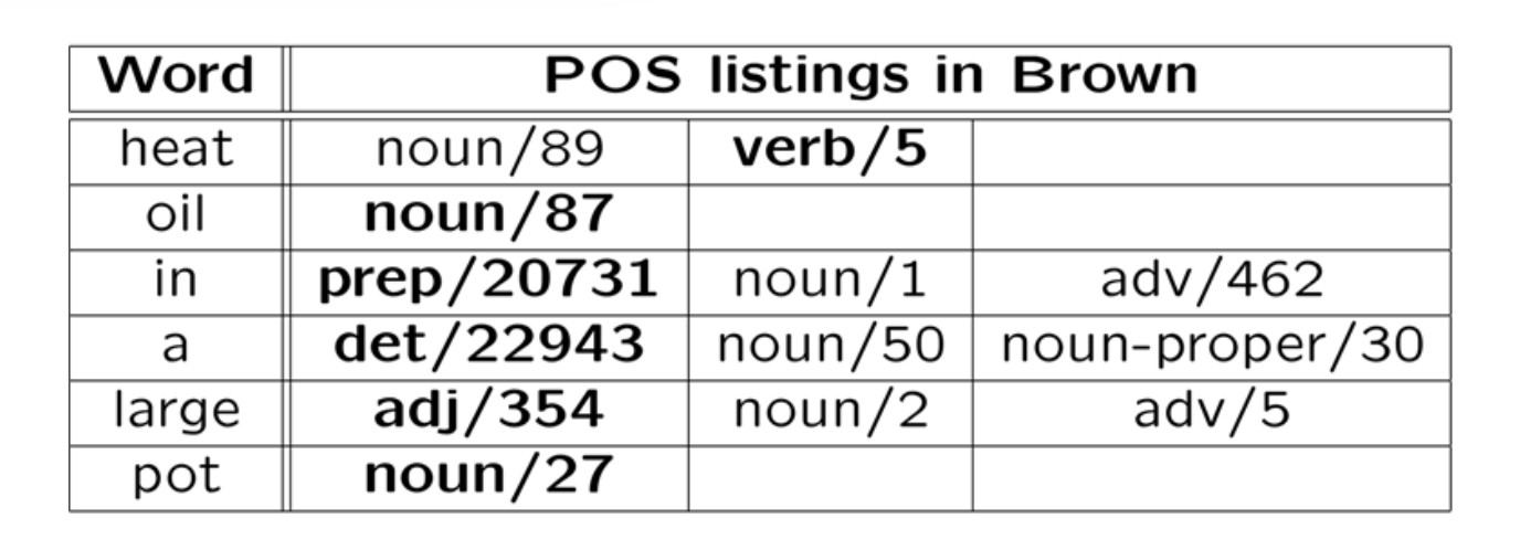
Consider the sentence "Heat oil in a large pot." The correct tag sequence is "verb noun prep det adj noun". Here's the tags seen when training on the Brown corpus.

(from Mitch Marcus)

Notice that

• individual words often have more than one plausible tag
• most commonly seen tag may not be correct choice for analyzing any particular input
• word may have possible tags that weren't seen in our training input (e.g. American training text might never include "over" used as a noun, a common cricket term)

Baseline algorithm

Most testing starts with a "baseline" algorithm, i.e. a simple method that does do the job, but typically not very well. In this case, our baseline algorithm might pick the most common tag for each word, ignoring context. In the table above, the most common tag for each word is shown in bold: it made one error out of six words.

The test/development data will typically contain some words that weren't seen in the training data. The baseline algorithm guesses that these are nouns, since that's the most common tag for infrequent words. An algorithm can figure this out by examining new words that appear in the development set, or by examining the set of words that occur only once in the training data ("hapax") words.

On larger tests, this baseline algorithm has an accuracy around 91%. It's essential for a proposed new algorithm to beat the baseline. In this case, that's not so easy because the baseline performance is unusually high.

Formulating the estimation problem

Suppose that W is our input word sequence (e.g. a sentence) and T is an input tag sequence. That is

$W = w_1, w_2, \ldots w_n$
$T = t_1, t_2, \ldots t_n$

Our goal is to find a tag sequence T that maximizes P(T | W). Using Bayes rule, this is equivalent to maximizing $P(W \mid T) * P(T)/P(W)$ And this is equivalent to maximizing $P(W \mid T) * P(T)$ because P(W) doesn't depend on T.

So we need to estimate P(W | T) and P(T) for one fixed word sequence W but for all choices for the tag sequenceT.

What can we realistically estimate?

Obviously we can't directly measure the probability of an entire sentence given a similarly long tag sequence. Using (say) the Brown corpus, we can get reasonable estimates for

• individual word frequencies
• tag usage for each word
• tag bigrams

If we have enough tagged data, we can also estimate tag trigrams. Tagged data is hard to get in quantity, because human intervention is needed for checking and correction.

Markov assumptions

To simplify the problem, we make "Markov assumptions." A Markov assumption is that the value of interest depends only on a short window of context. For example, we might assume that the probability of the next word depends only on the two previous words. You'll often see "Markov assumption" defined to allow only a single item of context. However, short finite contexts can easily be simulated using one-item contexts.

For POS tagging, we make two Markov assumptions. For each position k:

$P(w_k)$ depends only on $P(t_k)$
$P(t_k)$ depends only on $P(t_{k-1}$

Therefore

$P(W \mid T) = \prod_{i=1}^n P(w_i \mid t_i)$
$P(T) = P(t_1 | START) * \prod_{i=1}^n P(t_k \mid t_{k-1})$

where $P(t_1 | START)$ is the probability of tag $t_1$ at the start of a sentence.

HMM picture

Like Bayes nets, HMMs are a type of graphical model and so we can use similar pictures to visualize the statistical dependencies:

In this case, we have a sequence of tags at the top. Each tag depends only on the previous tag. Each word (bottom row) depends only on the corresonding tag.

AI in action