Since this class depends on data structures, which has discrete math as a prerequisite, most people have probably seen some version of BFS, DFS, and state graphs before. If this isn't true for you, this lecture probably went too fast. Aside from the textbook, you may wish to browse web pages for CS 173, CS 225, and/or web tutorials on BFS/DFS.
Key parts of a state graph:
Task: find a low-cost path from start state to a goal state.
Some applications want a minimum-cost path. Others may be ok with a path whose cost isn't stupidly bad (e.g. no loops).
We can take a real-world map (below left) and turn it into a graph (below right). Notice that the graph is not even close to being a tree. So search algorithms have to actively prevent looping, e.g. by remember which locations they've already visited.
Mapping this onto a state graph:
On the graph, it's easy to see that there are many paths from
Northampton to Amherst, e.g. 8 miles via Hadley,
31 miles via Williamsburg and Whately.
Left below is an ASCII maze of the sort used in 1980's computer games.
R is the robot, G is the goal, F is a food pellet to collect
on the way to the goal. We no longer play games of this style,
but you can still find search problems with this kind of simple
structure. On the right is one path to the goal. Notice that
it has to double back on itself in two places.
Modelling this as a state graph:
Some mazes impose tight constraints on where the robot can go,
e.g. the bottom corridor in the above maze is only one cell wide.
Mazes with large open areas can have vast numbers of possible
solutions. For example, the maze below has many paths from start to
goal. In this case, the robot needs to move 10 steps right and 10
steps down. Since there are no walls constraining the order of right
vs. downward moves, there are \(20 \choose 10 \) paths of shortest
length (20 steps), which is about 185,000 paths.
We need to quickly choose one of these paths rather than wasting
time exploring all of them individually.
Game mazes also illustrate another feature that appears in some AI
problems: the AI gains access to the state graph as it explores.
E.g. at the start of the game, the map may actually look like this:
States may also be descriptins of the real world in terms of feature values.
For example, consider the
Missionaries and Cannibals puzzle. In the starting state, there
are three missionaries, three cannibals, and a boat on the left side of a
river. We need to move all six people to the right side, subject to
the following constraints:
The state of the world can be described by three variables: how many missionaries on
the left bank, how many cannibals on the left bank, and which bank the boat is on.
The state space is shown below:
In this example
In speech recognition, we need to transcribe an acoustic waveform into
to produce written text. We'll see details of this process later in the
course. For now, just notice that this proceeds word-by-word.
So we have a set of candidate transcriptions for the first part of
the waveform and wish to extend those by one more word. For example,
one candidate transcription might start with "The book was very" and
the acoustic matcher says that the next word sounds like "short" or "sort."
In this example
Speech recognition systems have vast state spaces. A recognition
dictionary may know about 100,000 different words. Because acoustic
matching is still somewhat error-prone, there may be many words that
seem to match the next section of the input. So the
currently-relevant states are constructed on demand, as we search.
Chess is another example of an AI problem with a vast state space.
For all but the simplest AI problems, it's easy for a search algorithm to
get lost.
The first of these can send the program into an infinite loop. The
second and third can cause it to get lost, exploring states
very far from a reasonable path from the start to the goal.
Our first few search algorithms will be uninformed. That is, they
rely only on computed distances from the starting state. Next week,
we'll see \(A^*\)). It's an informed search algorithm because it
also uses an estimate of the distance remaining to reach the goal.
A state is exactly one of
Basic outline for search code
Data structure for frontier determines type of search
Let's find a route from Easthampton to Whately Using BFS.
The actual best route is via Northampton, Florence, Hatfield (19 miles)
The frontier is stored as a queue. So we explore locations in
rings, gradually moving outwards from the starting location.
Let's assume we always explore edges left to right.
We return the path Westhampton, Williamsburg, Whately (length 28)
BFS properties:
Here is a fun animation of
BFS set to music.
The frontier is stored as a stack (explicitly or implicitly via recursive function calls).
Again, we'll explore edges left to right. The frontier looks like:
We return the path: Westhampton, Chesterfield, Goshen, Whateley (length 38)
DFS properties:
Animation of
DFS set to music.
Compare this to the one for BFS.
When searching a large state space, there can be a huge number of seen
states. If states have to be instantiated for other reasons (e.g. a
full map is loaded into memory), this is not a problem because we can
simply add a mark bit to each state.
If states are generated dynamically, DFS can save a lot of memory as follows:
The cost is that this version of DFS does redundant work because it
has a poor memory for what it has already examined. This tradeoff
can be good or bad depending on the structure of the state space.
We can dramatically improve the low-memory version of DFS by
running it with a progressively increasing bound on the maximum path
length. That is
This is called "iterative deepening." Its properties
Each iteration repeats the work of the previous one. However,
the number of states increases very fast with depth. So running time
is dominated by work in the last iteration.
Mazes
Puzzle
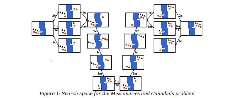 (from
Gerhard Wickler, U. Edinburgh)
(from
Gerhard Wickler, U. Edinburgh)
Speech recognition
Some high-level points
Basic search outline
Loop until we find a solution
BFS example
DFS example
Storing seen states
Iterative deepening
For k = 1 to infinity
Run DFS but stop whenever a path contains at least k states.
Halt when we find a goal state