Recap

We'd like to convert the context of a word w (aka words seen near w) to short, informative feature vectors. Previous methods did this in two steps:

• build and normalize long feature vectors, and then
• make them shorter and more dense.

word2vec (aka skip-gram) does this all in one step, i.e. directly learns how to embed words into an n-dimensional feature space.

Two similar embedding algorithms (which we won't cover) are the CBOW algorithm from word2vec and the GloVe algorithm from Stanford.

word2vec: overview

In broad outline word2vec has three steps

• Gather pairs (w,c) where w is our focus word and c is a nearby context word,
• Embed all words into k-dimensional space (e.g. randomly).
• Iteratively adjust the embedding so that pairs (w,c) end up with similar coordinates.

A pair (w,c) is considered "similar" if the dot product $w\cdot c$ is large.

For example, our initial random embedding might put "elephant" near "matchbox" and far from "rhino." Our iterative adjustment would gradually move the embedding for "rhino" nearer to the embedding for "elephant."

Two obvious parameters to select. The dimension of the embedding space would depend on how detailed a representation the end user wants. The size of the context window would be tuned for good performance.

Negative sampling

Problem: a great solution for the above optimization is to map all words to the same embedding vector. That defeats the purpose of having word embeddings.

If we had negative examples (w,c'), we could make the optimization move w and c' away from each other. Revised problem: our data doesn't provide negative examples.

Solution: Train against random noise, i.e. randomly generate "bad" context words for each focus word.

• called "negative sampling" (not a very evocative term)
• For a fixed focus word w, negative context words are picked with a probability based on how often words occur in the training data.
• depends on good examples being relatively sparse in the space of all word pairs (probably correct)

The negative training data will be corrupted by containing some good examples, but this corruption should be a small percentage of the negative training data.

Details of algorithm

Focus and context words are embedded independently into k-dimensional space. Since each word can (obviously) serve both functions, each word gets embedded twice, once for each role. A single embedding for both roles runs into the problem that each word w is not a common context for itself (e.g. "dog dog" isn't very common) but the dot product $w \cdot w$ ls large.

Our classifier tries to predict yes/no from pairs (w,c).

We'd like to make this into a probabilistic model. So we run dot product through a sigmoid to produce a "probability" that (w,c) is a good word-context pair. That is, we approximate

$P(\text{good} | w,c) \approx \sigma(w\cdot c).$

By the magic of exponentials (see below), this means that the probability that (w,c) is not a good word-context pair is

$P(\text{bad} | w,c) \approx \sigma(-w\cdot c).$

Suppose that D is the positive training pairs and D' is the set of negative training pairs. So our iterative refinement algorithm adjusts the embeddings (both context and word) so as to maximize

$\sum_{(w,c) in D} \ \sigma(w\cdot c) + \sum_{(w,c) in D'} \ \sigma(-w\cdot c)$

Unexplained exponentials

Ok, so how did we get from $P(\text{good} | w,c) = \sigma(w\cdot c)$ to $P(\text{bad} | w,c) = \sigma(-w\cdot c)$?

"Good" and "bad" are supposed to be opposites. So $P(\text{bad} | w,c) = \sigma(-w\cdot c)$ should be equal to $1 - P(\text{good}| w,c) = 1- \sigma(w\cdot c)$. I claim that $1 - \sigma(w\cdot c) = \sigma(-w\cdot c)$.

This claim actually has nothing to do with the dot products. As a general thing $1 - \sigma(x) = \sigma(-x)$. Here's the math.

Recall the definition of the sigmoid function: $\sigma(x) = \frac{1}{1+e^{-x}}$.

$\eqalign{ 1-\sigma(x) &=& 1 - \frac{1}{1+e^{-x}} = \frac{e^{-x}}{1+ e^{-x}} \ \ \text{ (add the fractions)} \\ &=& \frac{1}{1/e^{-x}+ 1} \ \ (\text{divide top and bottom by } e^{-x}) \\ &=& \frac{1}{e^x + 1} \ \ \text{(what does a negative exponent mean?)} \\ &=& \frac{1}{1 + e^x} = \sigma(-x)}$

Building the set of training examples

A number of other tweaks are required to get good performance out of word2vec. Some of these can also be used on some of the related models from the previous lecture.

Tweak 1: Postive training examples are weighted by 1/m, where m is the distance between the focus and context word. I.e. so adjacent context words are more important than words with a bit of separation.

Tweak 2: Word2vec uses more negative training examples than positive examples, by a factor of 2 up to 20 (depending on the amount of training data available).

Smoothing negative context counts

For a fixed focus word w, negative context words are picked with a probability based on how often words occur in the training data. However, if we compute P(c) = count(c)/N (N is total words in data), rare words aren't picked often enough as context words. So instead we replace each raw count count(c) with $(\text{count}(c))^\alpha$. The probabilities used for selecting negative training examples are computed from these smoothed counts.

$\alpha$ is usually set to 0.75. But to see how this brings up the probabilities of rare words, set $\alpha = 0.5$, i.e. we're computing the square root of the input: In the table below, you can see that large probabilities stay large, but very small ones are increased by quite a lot.

x	$\sqrt{x}$
.99	.995
.9	.95
.1	.3
.01	.1
.0001	.01

This trick can also be used on PMI values (e.g. if using the methods from the previous lecture).

Delection, subsampling

Ah, but apparently they are still unhappy with the treatment of very common and very rare words. So, when we first read the input training data, word2vec modifies it as follows:

• very rare words are deleted from the text, and
• very common words are deleted with a probability that increases with how frequent they are.

This improves the balance between rare and common words. Also, deleting a word brings the other words closer together, which improves the effectiveness of our context windows.

Modelling analogies, compositional semantics

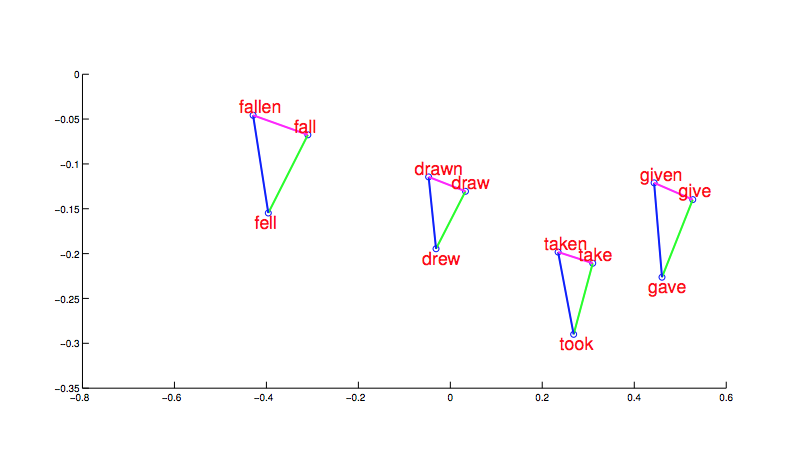
Even the final word embeddings still involve vectors that are too long to display conveniently. Projections onto two dimensions (or three dimensions with moving videos) are hard to evaluate. More convincing evidence for the coherency of the output comes from word relationships. First, notice that morphologically related words end up clustered. And, more interesting, the shape and position of the clusters are the same for different stems.

from Mikolov, NIPS 2014

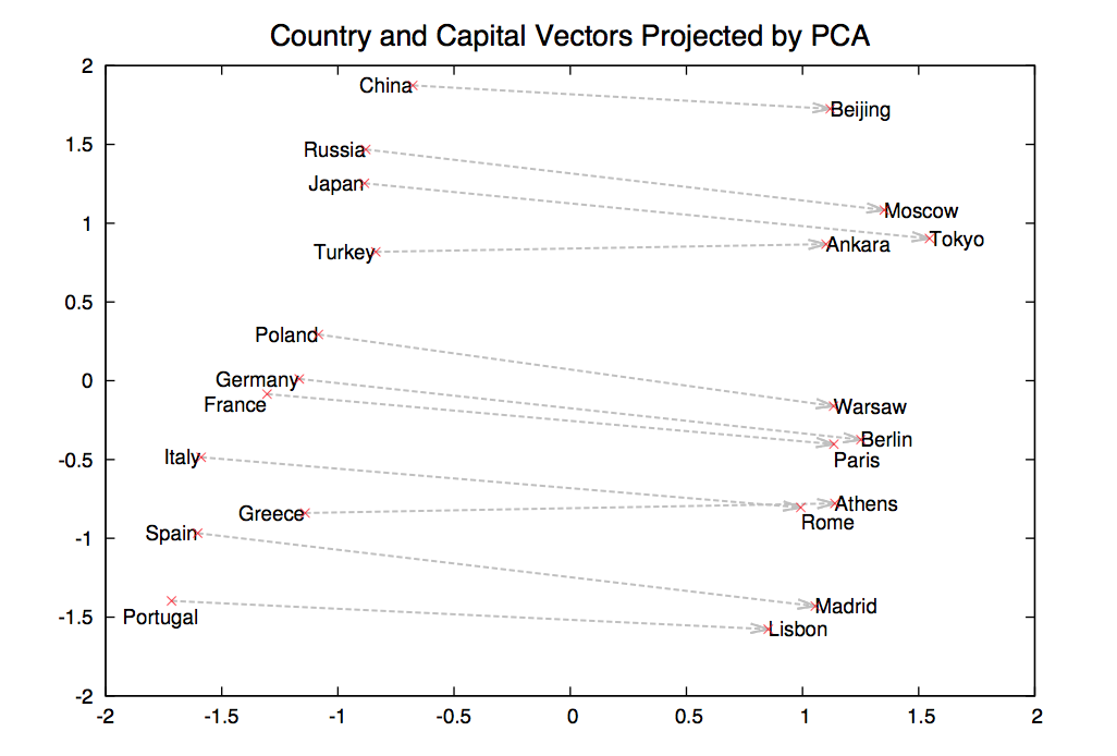
Now suppose we find a bunch of pairs of words illustrating a common relation, e.g. countries and their capitals in the figure below. The vectors relating the first word (country) to the second word (capital) all go roughly in the same direction.

from Mikolov, NIPS 2014

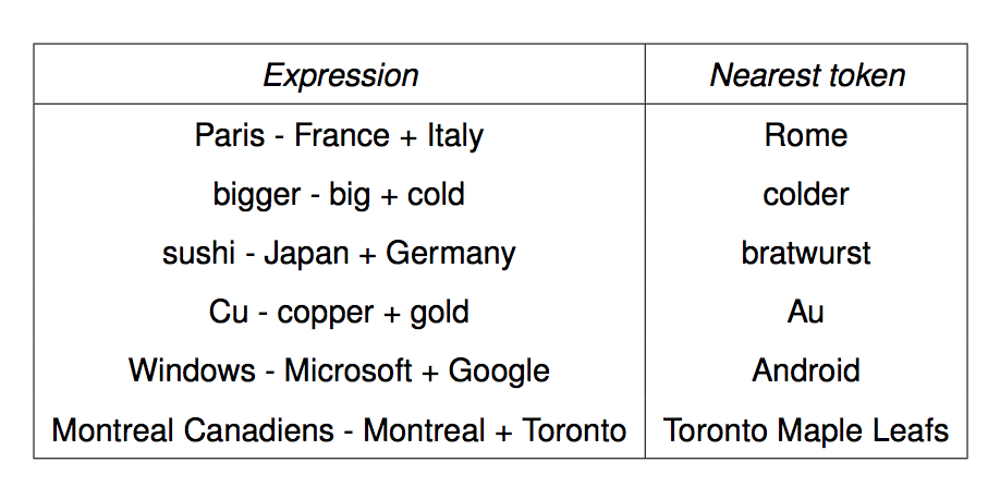
We can get the meaning of a short phrase by adding up the vectors for the words it contains. But we can also do simple analogical reasoning by vector addition and subtraction. So if we add up

vector("Paris") - vector("France") + vector("Italy")

We should get the answer to the analogy question "Paris is to France as ?? is to Italy". The table below shows examples where this calculation produced an embedding vector close to the right answer:

from Mikolov, NIPS 2014

How much data?

The embedding results shown above (from 2014) use 1 billion words to train embeddings for basic task.

For the word analogy tasks, they used an embedding with 1000 dimensions and about 33 billion words of training data. Performance on word analogies is about 66%.

Comparison: children hear about 2-10 million words per year. Assuming the high end of that range of estimates, they've heard about 170 million words by the time they take the SAT. So the algorithm is performing well, but still seems to be underperforming given the amount of data it's consuming.

Some follow-on papers

Original Mikolov et all papers:

• Efficient Estimation of Word Representations in Vector Space
• Distributed Representations of Words and Phrases and their Compositionality

Goldberg and Levy papers (easier and more explicit)

• word2vec Explained
• Dependency-Based Word Embeddings
• Neural Word Embedding as Implicit Matrix Factorization
• Improving Distributional Similarity with Lessons learned from Word Embeddings

AI in action

New ISS companion robot