Recap

Vector models of meaning

• meanings of a word using a vector of what words it occurs near.
• topic of a document using what words appear in it.

For example, we might use the following counts of which words appear in which Shakespeare plays. This 2D table can be seen as vectors representing documents in terms of word counts, or as vectors representing words in terms of context documents.

Normalizing word counts

Raw word count vectors don't work very well. Issues:

• The raw counts require normalization.
• Vectors are too long and too sparse.

Why do the counts need normalization?

• rare words have fewer observations than common ones and, similarly, short documents have fewer words than longer ones
• very frequent words aren't useful context
• local observations (e.g. within a document) are highly correlated
• rare words provide unreliable context

So we'll need to

• normalize the counts
• map the vectors into a lower-dimensional space

We'll first see older methods in which these two steps are distinct. Word2vec (next lecture) accomplishes both via one procedure.

TF-IDF

TF-IDF normalization addresses the problem that

• very frequent words aren't useful context
• local observations (e.g. within a document) are highly correlated

It is a bit of a hack, but one that has proved very useful in document retrieval.

Suppose that we are looking at a particular focus word in a particular focus document. The TF-IDF feature is the product of TF (normalized word count) and IDF (inverse document frequency).

To compute TF, we smooth the raw count c for the word.

TF = $1+\log_{10}(c)$, if count > 0
TF = 0, if count = 0

The document frequency (DF) of the word, is df/N, where N is the total number of documents and df is the number our word appears in. When DF is small, our word provides a lot of information about the topic. When DF is large, our word is used in a lot of different contexts and so provides little information about the topic.

The normalizing factor IDF is computed as

IDF = $\log_{10}(N/df)$

That is, we invert DF and estimate the importance of the numbers using a log scale. This is partly motivated by the fact that human perceptions of intensity or quantity are often well modelled by a log scale.

The final number that goes into our vector representation is TF*IDF. That is, we multiply the two quantities even though we've already put them both onto a log scale.

How similar are two documents?

Suppose we have a feature vector for each document (e.g. from TF-IDF). ach document has a vector of word counts (normalized as in TF-IDF) How do we measure similarity between documents?

Notice that short documents have fewer words than longer ones. And, later on, we'll run into the similar issue that rare words have fewer observations than common ones. So we normally consider only the direction of these feature vectors, not their lengths. So

(2, 1, 0, 4, ...)
(6, 3, 0, 8, ...) same as previous
(2, 3, 1, 2, ...) different

Basic idea: we're measuring the angle between the two vectors.

Forgotten linear algebra

The actual angle is hard to work with, e.g. we can't compute it without calling an inverse trig function. It's much easier to approximate this with the cosine of the angle.

Recall what the cosine function looks like

• 1 at 0 degrees (i.e. the two vectors match)
• 0 at 90 degrees (i.e. the two vectors are perpendicular)

What happens past 90 degrees? Oh, word counts can't be negative! So our vectors all live in the first quadrant and can't differ by more than 90 degrees.

Recall a handy formula for computing the cosine of the angle $\theta$ between two vectors:

input vectors $v = (v_1,v_2,\ldots,v_n)$ and $w = (w_1,w_2,\ldots,w_n)$
dot product: $v\cdot w = v_1w_1 + ... + v_nw_n$
$\cos(\theta) = \frac{v \cdot w}{|v||w|}$

So you'll see both "cosine" and "dot product" used to describe this measure of similarity.

Pointwise mutual information (PMI)

Let's switch to our other example of feature vectors: modelling a word's meaning on the basis of words seen near it in running text. We still have the same kinds of normalization/smoothing issues.

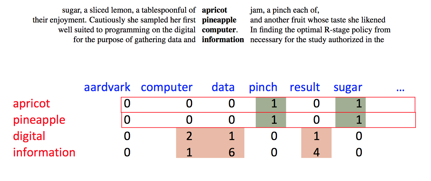
Here's a different (but also long-standing) approach to normalization. We've picked a focus word w and a context word c. We'd like to know how closely our two words are connected. That is, do they occur together more often than one might expect for independent draws?

Suppose that w occurs with probability P(w) and c with probability P(c). If the two were appearing independently in the text, the probability of seeing them together would be P(w)P(c). Our actual observed probability is P(w,c). So we can use the following fraction to gauge how far away they are from independent:

$\frac {P(w,c)}{P(w)P(c)}$

Example: consider "of the" and "three-toed sloth." The former occurs a lot more often. However, that's mostly because its two constituent words are both very frequent. The PMI normalizes by the frequencies of the constituent words.

Putting this on a log scale gives us the pointwise mutual information (PMI)

$I(w,c) = \log_2(\frac {P(w,c)}{P(w)P(c)})$

When one or both words are rare, there is high sampling error in their probabilities. E.g. if we've seen a word only once, we don't know if it occurs once in 10,000 words or once in 1 million words. So negative values of PMI are frequently not reliable. This observation leads some researchers to use the positive PMI (PPMI):

PPMI = max(0,PMI)

Warning: negative PMI values may be statistically significant, and informative in practice, if both words are quite common. For example, "the of" is infrequent because it violates English grammar. There have been some computational linguistics algorithms that exploit these significant zeroes.

Singular value decomposition (SVD)

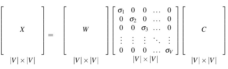
Both TF-IDF and PMI methods create vectors that contain informative numbers but are very long and sparse. For most applications, we would like to reduce these to short dense vectors that capture the most important dimensions of variation. A traditional method of doing this uses the singular value decomposition (SVD).

Theorem: any rectangular matrix can be decomposed into three matrices:

• W: maps original coordinates into new ones
• S: diagonal matrix of "singular values"
• C: maps new coordinates back to original ones

from Dan Jurafsky at Stanford.

In the new coordinate system (the input/output of the S matrix), the information in our original vectors is represented by a set of orthogonal vectors. The values in the S matrix tell you how important each basis vector is, for representing the data. We can make it so that weights in S are in decreasing order top to bottom.

It is well-known how to compute this decomposition. See a scientific computing text for methods to do it accurately and fast. Or, much better, get a standard statistics or numerical analysis package to do the work for you.

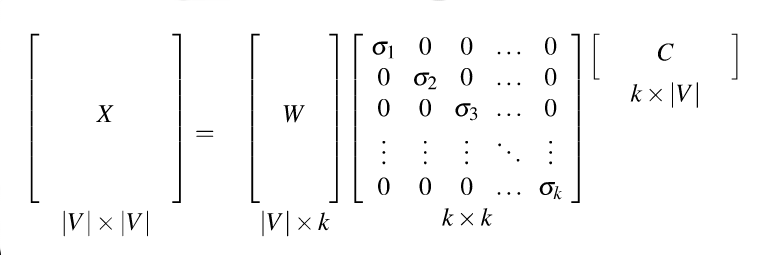
Recall that our goal was to create shorter vectors. The most important information lies in the top-left part of the S matrix, where the S values are high. So let's consider only the top k dimensions from our new coordinate system: The matrix W tells us how to map our input sparse feature vectors into these k-dimensional dense feature vectors.

from Dan Jurafsky at Stanford.

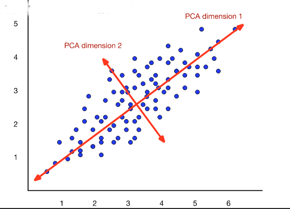
The new dimensions are called the "principal components." So this technique is often called a principal component analysis (PCA). When this approach is applied to analysis of document topics, it is often called "latent semantic analysis" (LSA).

from Dan Jurafsky at Stanford.

Bottom line on SVD/PCA

• Been around for ages. Lots of packages to do it for you.
• Helps human analysts figure out the important dimensions of variation.
• Works pretty well. Only the best newer methods do better.

AI in action

AI systems imitate biases found in their training data.