We've see model-based reinforcement learning. Let's now look at model-free learning. For reasons that will become obvious, this is also known as Q-learning.

A useful tutorial from Travis DeWolf:

• Q learning
• SARSA vs. Q learning

Recap: Bellman equation

$U(s) = R(s) + \gamma \max_a \sum_{s'} P(s' | s,a)U(s')$

Where

• s is the current state
• a is the commanded action
• s' is new state we actually end up in

Model-free reinforcement learning (aka Q-learning)

For Q learning, we split up and recombine the Bellman equation. First, notice that we can rewrite the equation as follows, because $\gamma$ is a constant and R(s) doesn't depend on which action we choose in the maximization.

$U(s) = \max_a [\ R(s) + \gamma \sum_{s'} P(s' | s,a)U(s')\ ]$

Then divide the equation into two parts:

• $Q(s,a) = R(s) + \gamma \sum_{s'} P(s' | s, a) U(s')$
• $U(s) = \max_a Q(s,a)$

Q(s,a) tells us the value of commanding action a when the agent is in state s. Q(s,a) is much like U(s), except that the action is fixed via an input argument. As we'll see below, we can directly estimate Q(s,a) based on experience.

To get the analog of the Bellman equation for Q values, we recombine the two sections of the Bellman equation in the opposite order. So change variables in the second equation:

$U(s') = \max_{a'} Q(s',a')$

Then substitute the second equation into the first

$Q(s,a) = R(s) + \gamma \sum_{s'} P(s' | s, a) \max_{a'\in A} Q(s',a')$

This formulation entirely removes the utility function U in favor of the function Q. But we still have an inconvenient dependence on the transition probabilities P.

Removing the transition probabilities

To figure out how to remove the transition probabilities from our update equation, assume we're looking at one fixed choice of state s and commanded action a and consider just the critical inner part of the expression:

$\sum_{s'} P(s' | s, a) \max_{a'} Q(s',a')$

We're weighting the value of each possible next state s' by the probability P(s' | s,a) that it will happen when we command action a in state s.

Suppose that we command action a from state s many times. For example, we roam around our environment, occasionally returning to state s. Then, over time, we'll transition into s' a number of times proportional to its transition probability P(s' | s,a). So if we just average

$\max_{a'} Q(s',a')$

over an extended sequence of actions, we'll get an estimate of

$\sum_{s'} P(s' | s, a) \max_{a'} Q(s',a')$

So we can estimate Q(s,a) by averaging the following quantity over an extended sequence of timesteps t

$Q_t(s,a) = R(s) + \gamma \max_{a'} Q(s',a')$

We need these estimates for all pairs of state and action. In a realistic training sequence, we'll move from state to state, but keep returning periodically to each state. So this averaging process should still work, as long as we do enough exploration.

Q-value update equations

The above assumes implicitly that we have a finite sequence of training data, processed as a batch, so that we can average up groups of values in the obvious way. How do we do this incrementally as the agent moves around?

One way to calculate the average of a series of values $V_1 \ldots V_n$ is to start with an initial estimate of zero and average in each incoming value with a an appropriate discount. That is

• V = 0
• loop for t=1 to n
  • $V = V + V_t/n$

Now suppose that we have an ongoing sequence with no obvious endpoint. Or perhaps the sequence is so long that the world might gradually change, so we'd like to slowly adapt to change. Then we can do a similar calculation called a moving average:

• V = 0
• loop for t=1 to forever
  • V = $(1-\alpha) V + \alpha V_t$

The influence of each input decays gradually over time. The effective size of the averaging window depends on the constant $\alpha$.

If we use this to average our values Q_t(s,a), we get an update method that looks like:

• Q(s,a) = 0 for all s and all a
• for t = 1 to forever
  • $Q(s,a) = (1-\alpha) Q(s,a) + \alpha [R(s) + \gamma \max_{a'} Q(s',a')]$

Our update equation can also be written as

$Q(s,a) = Q(s,a) + \alpha [R(s) - Q(s,a) + \gamma \max_{a'} Q(s',a')]$

Temporal difference (TD) learning

We can now set up the full "temporal difference" algorithm for choosing actions while learning the Q values.

• Q(s,a) = 0 for all s and all a
• for t = 1 to forever
  1. in the current state s, select an action a
  2. observe the reward R(s) and the next state s'
  3. update our Q values $Q(s,a) = Q(s,a) + \alpha [R(s) - Q(s,a) + \gamma \max_{a'} Q(s',a')]$

The obvious choice for an action to command in step 1 is

$\pi(s) = \text{argmax}_{a} Q(s,a)$

But recall from last lecture that the agent also needs to explore. So a better method is

• Sometimes choose $\pi(s) = \text{argmax}_{a} Q(s,a)$
• Otherwise choose a random or semi-random exploration state.

This creates an inconsistency in our algorithm.

• The maximization $\max_{a'} Q(s',a')$ in step 3 assumes we pick the action that will yield the highest value, but
• Step 1 doesn't always choose the action that currently seems to have the highest value.

So the update in step 3 is based on a different action from the one actually chosen by the agent.

SARSA

The SARSA ("State-Action-Reward-State-Action") algorithm adjusts the TD algorithm to align the update with the actual choice of action. The algorithm looks like this, where (s,a) is our current state and action and (s',a') is the following state and action.

• pick an initial state s and initial action a
• for t = 1 to forever
  • observe the reward R(s) and the next state s'
  • from next state s', select next action a'
  • update our Q values using $Q(s,a) = Q(s,a) + \alpha [R(s) - Q(s,a) + \gamma Q(s',a')]$
  • (s,a) = (s',a')

So we're unrolling a bit more of the state-action sequence before doing the update, and our updates always use the actions that the agent chose.

SARSA vs. TD update

Here's an example from Travis DeWolf that nicely illustrates the difference between SARSA and TD update. The agent is prone to occasional random motions, because it likes to explore rather than just following its optimal policy. The TD algorithm assumes it will do a better job of following policy, so it sends the agent along the edge of the hazard and it regularly falls in. The SARSA agent stays further from the hazard, so that the occasional random motion isn't likely to be damaging.

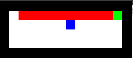Mouse (blue) tries to get cheese (green) without falling in the pit of fire (red).

Trained using TD update

Trained using SARSA

Tweaks and extensions

There are many variations on reinforcement learning. Especially interesting ones include

• use features to model states, so we can predict values for unseen states
• deploy deep learning
• imitate an expert rather than having numerical rewards.

Reinforcement Learning Demos and Applications

Stanford helicopter

Spider robot from Yamabuchi et al 2013

playing Atari games (V. Mnih et al, Nature, February 2015)

Alphago

• from Google's Deepmind
• how it works

AI in action

Reinforcement learning code learns how to cheat at games.