Credits to Matt Gormley are from 10-601 CMU 2017

Hidden layers

So far, we've seen some systems containing more than one classifier unit, but each unit was always directly connected to the inputs and an output. When people say "neural net," they usually mean a design with more than layer of units, including "hidden" units which aren't directly connected to the output.

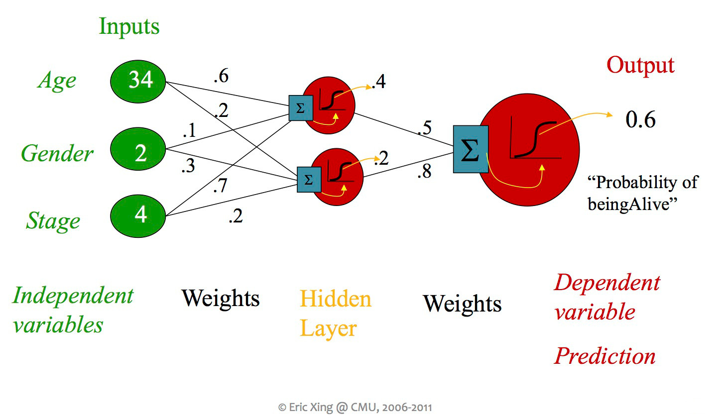
from Eric Xing via Matt Gormley

A single unit in a neural net can look like any of the linear classifiers we've seen previously. Moreover, different layers within a neural net design may use types of units (e.g. different activation functions).

from Matt Gormley

Approximating functions

In theory, a single hidden layer is sufficient to approximate any continuous function, assuming you have enough hidden units. However, deeper neural nets seem to be easier to design and train. These deep networks normally emulate the layers of processing found in previous human-designed classifiers. So each layer transforms the input so as to make it more sophisticated ("high level"), compacts large inputs (e.g. huge pictures) into a more manageable set of features, etc. The picture below shows a face recognizer in which the bottom units detect edges, later units detect small pieces of the face (e.g. eyes), and the last level (before the output) finds faces.

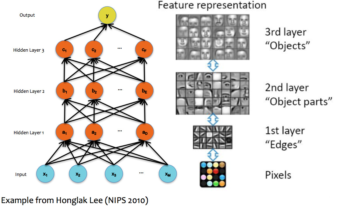
(from Matt Gormley)

Approximating functions

Here are some slides showing how a neural net with increasingly many layers can approximate increasingly complex decision boundaries. (from Eric Postma via Jason Eisner via Matt Gormley)

To approximate a complex shape with onlyl 2-3 layers, each hidden unit takes on some limited task. For example, one unit may define the top edge of a set of examples lying in a band:

• Approximating a diagonal band (from Matt Gormley)
• Approximating a "pocket" (from Matt Gormley)

More complex shapes such as this two "pocket" region (pictures from Matt Gormley) require increasingly many layers. Notice that the second picture shows k-nearest neighbors on the same set of data.

Training

Neural nets are trained in much the same way as individual classifiers. That is, we initialize the weights, then sweep through the input data multiple types updating the weights. Each update for a weight $w_i$ should look like

$w_i = w_i - \alpha * \frac{\partial \text{ loss}}{\partial w_i}$

One new issue in training is symmetry breaking. That is, we need to ensure that hidden units in the same layer learn to do different things. Suppose that two units have the same inputs, and also send their output to the same place(s). Then our basic linear classifier training will give them the same weights. At that point, they will do the same thing, so we might as well just have one unit. Two approaches to symmetry breaking:

• Set the initial weights to random values.
• Randomize some aspect of the later training, e.g. ignore some randomly-chosen units on each update.

A second issue is that our linear classifier update rule depended upon being able to directly see the input values and the output loss. One or both of these will be impossible for units in a multi-layer network. So we use a two-pass update procedure:

• Forward: starting from the network inputs, working forwards through the network, and using our current weights, calculate the output values for all units.
• Find the loss at the end (with the current weights).
• Backpropagation: starting from the loss at the end of the network and working backwards, calculate how changes to each weight will affect the loss.

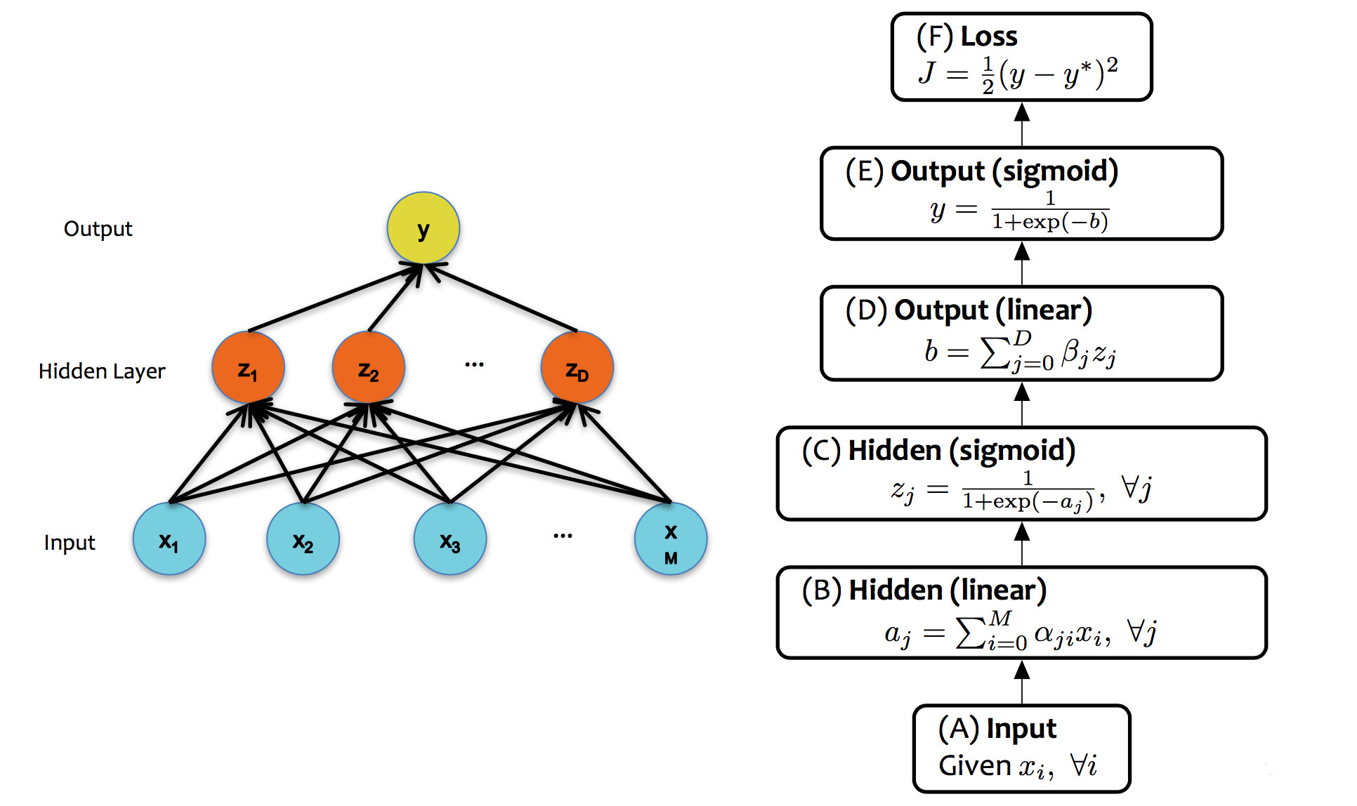
The forward pass does exactly what you'd think.

Backpropagation

Backpropagation is essentially a mechanical exercise in applying the chain rule repeatedly. Humans make mistakes, and direct manual coding will have bugs. So, as you might expect, computers have taken over most of the work as they for (say) register allocation. Read the very tiny example in Jurafsky and Martin (7.4.3 and 7.4.4) to get a sense of the process, but then assume you'll use TensorFlow or PyTorch to make this happen for a real network.

Here's the basic idea. If $h(x) = f(g(x))$, the chain rule says that $h'(x) = f'(g(x))*g'(x)$. In other words, to compute $h'(x)$, we'll need the derivatives of the two individual functions, plus the value of of them applied to the input. Forward values such as g(x) are produced by the initial forward pass in the updating algorithm. Backpropagation fills in the derivative values.

Let's write out the same thing in Liebniz notation, with some explicit variables for the intermediate results:

• y = g(x)
• z = f(y) = f(g(x))
• $\frac{dh}{dx} = \frac{df}{dy} * \frac{dg}{dx}$

This version tends to hide the fact that we need the values from the forward pass. However, we can now see that the derivative for a whole composed chain of functions is, essentially, the product of the derivatives for the individual functions. So, for a weight w at some level of the network, we can assemble the value for $\frac{d\text{ loss}}{dw}$ using the equation for the derivative at our level plus the derivative values computed at the previous level.

The diagram below shows the forward and backward values for the example net near the start of this lecture.

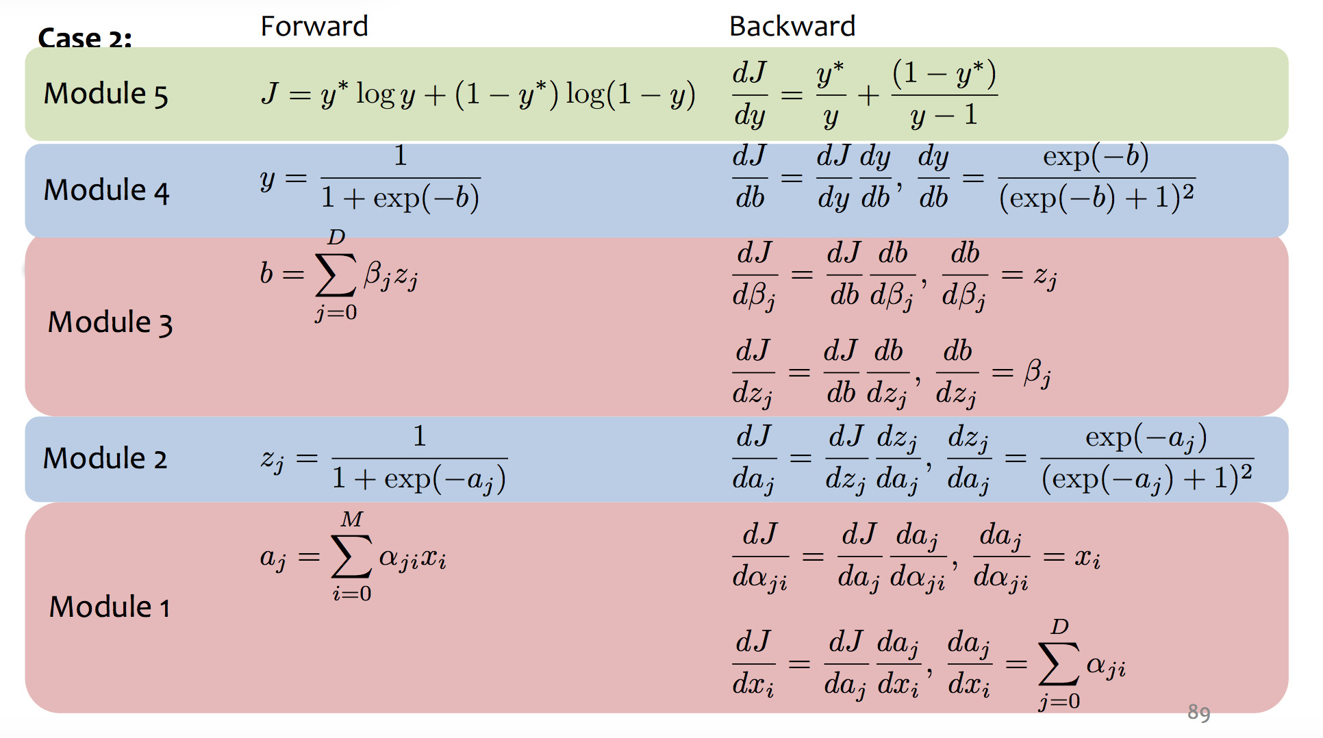(from Matt Gormley)

AI in action

A project to physically model networks of neurons.